Creating a Restaurant Robot Simulation, Part 1- #ROS Projects
.
What we are going to learn
- How to add modifications to the 3D model.
- How to create a load sensor plugin for gazebo.
- How to set up navigation, create a map and save table waypoints.
In summary, we will learn how to create a simulation that allows us to simulate a robot that serves in a restaurant.
List of resources used in this post
- ROSject containing all the code used in this post, including simulations, ready to be executed: http://www.rosject.io/l/ded2912/
- Related ROS courses:
- 1. URDF for Robot Modeling
- 2. Creating Web interfaces for ROS robots
- 3. Create Your First Robot With ROS
- BOM:
- 3D Models of apple: https://www.blendswap.com/blend/23583
- DroidSpeak: https://gitlab.com/easymov/droidspeak
- Barista code in BitBucket: https://bitbucket.org/theconstructcore/barista_systems/src/master/
Open the ROSject
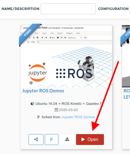
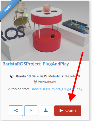
In order to see the simulation, you have to click on the ROSject link (http://www.rosject.io/l/ded2912/) to get a copy of the ROSject. You can now open the ROSject by clicking on the Open ROSject button.
Open ROSject – Barista Robot
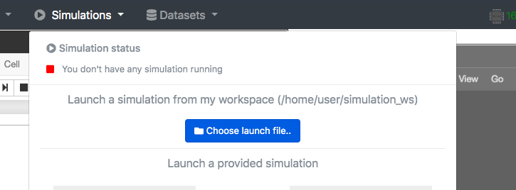
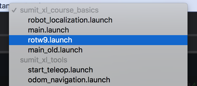
Launching the simulation
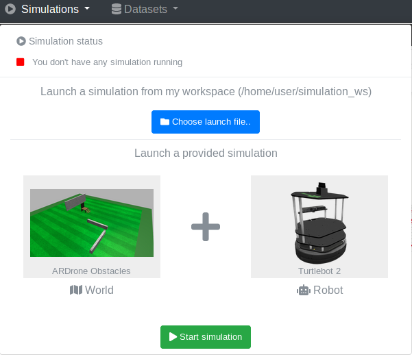
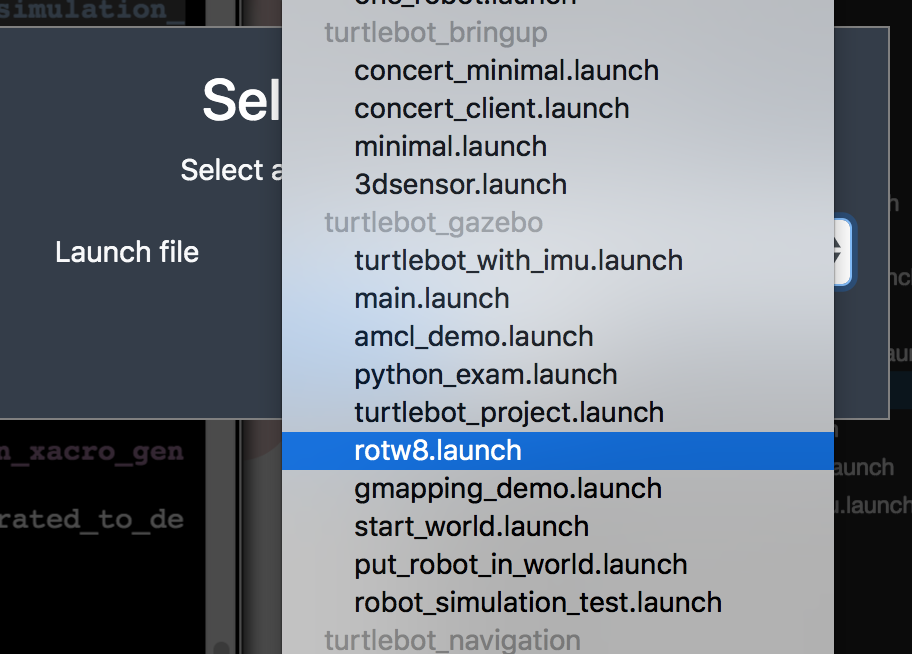
With the ROSject open, you can launch the simulation by clicking Simulation, then Choose Launch File. Then you select the main_simple.launch file from the barista_gazebo package.
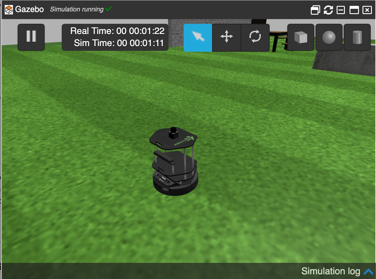
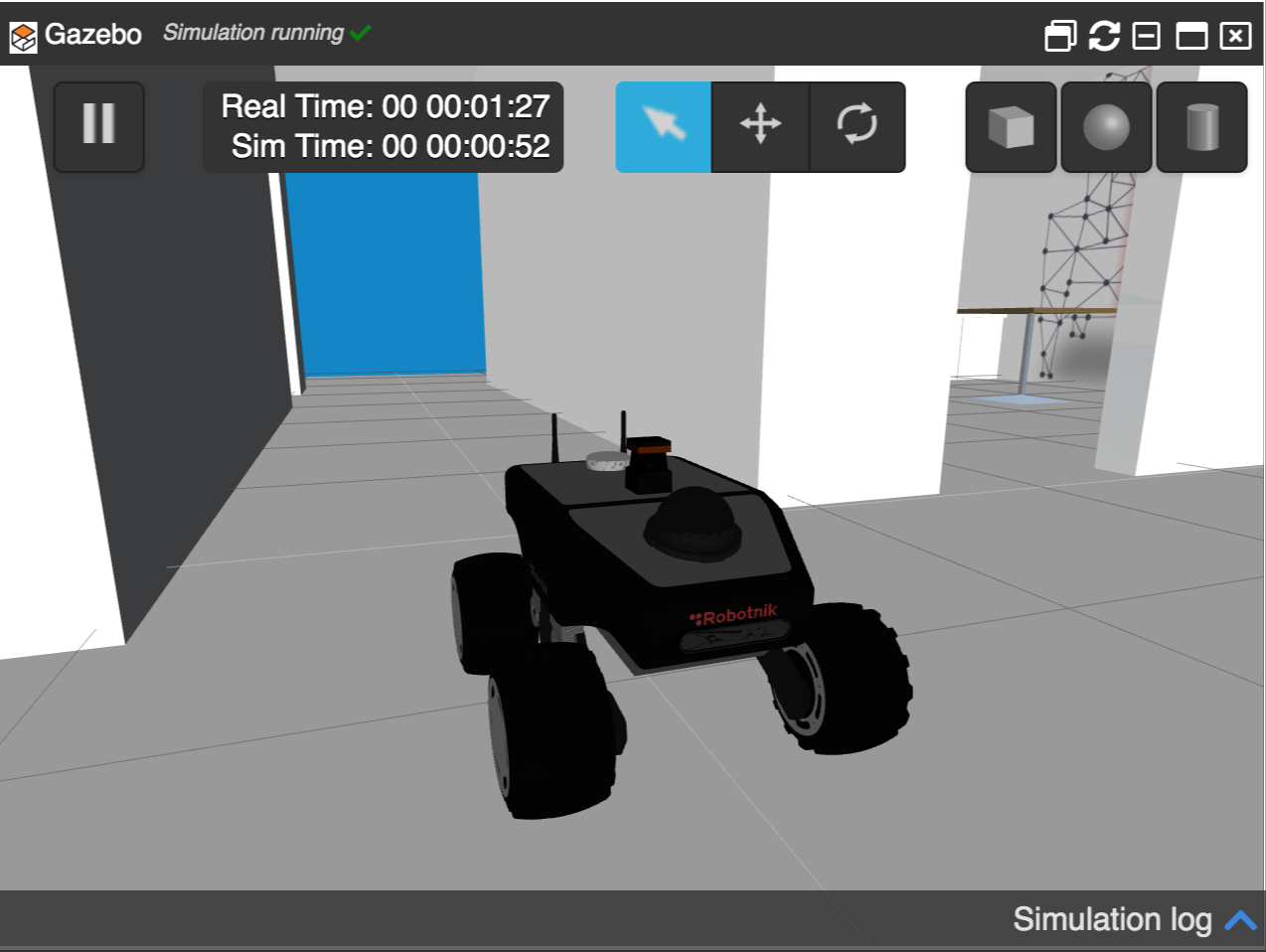
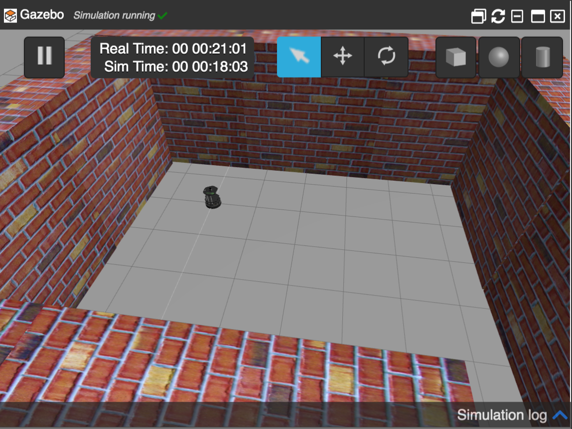
If everything went ok, you should now have the simulation like in the image below:
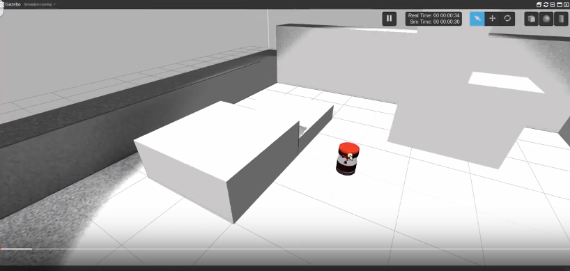
Barista Robot in ROSDS
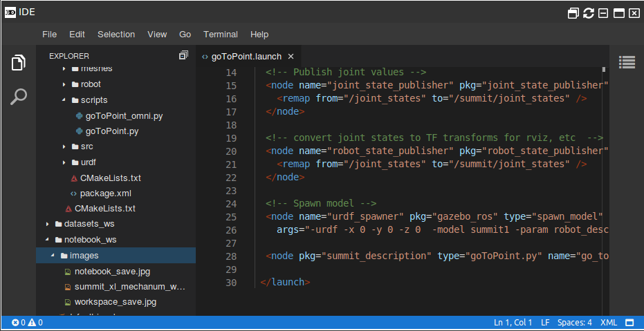
The launch file we just selected can be found on ~/simulation_ws/src/barista/barista_gazebo/launch/main_simple.launch and has the following content:
<?xml version="1.0" encoding="UTF-8"?>
<launch>
  <arg name="pause" default="false"/>
  <arg name="x" default="0"/>
  <arg name="y" default="0"/>
  <arg name="z" default="0.0"/>
  <arg name="roll" default="0"/>
  <arg name="pitch" default="0"/>
  <arg name="yaw" default="0" />

  <include file="$(find barista_worlds)/launch/start_world_simple10x10.launch">
    <arg name="pause" value="$(arg pause)" />

    <arg name="put_robot_in_world" value="true" />
    <arg name="put_robot_in_world_package" value="barista_gazebo" />
    <arg name="put_robot_in_world_launch" value="put_robot_in_world.launch" />

    <arg name="x" value="$(arg x)" />
    <arg name="y" value="$(arg y)" />
    <arg name="z" value="$(arg z)" />
    <arg name="roll" value="$(arg roll)"/>
    <arg name="pitch" value="$(arg pitch)"/>
    <arg name="yaw" value="$(arg yaw)"/>
  </include>

  <include file="$(find barista_description)/launch/rviz_localization.launch"/>


</launch>
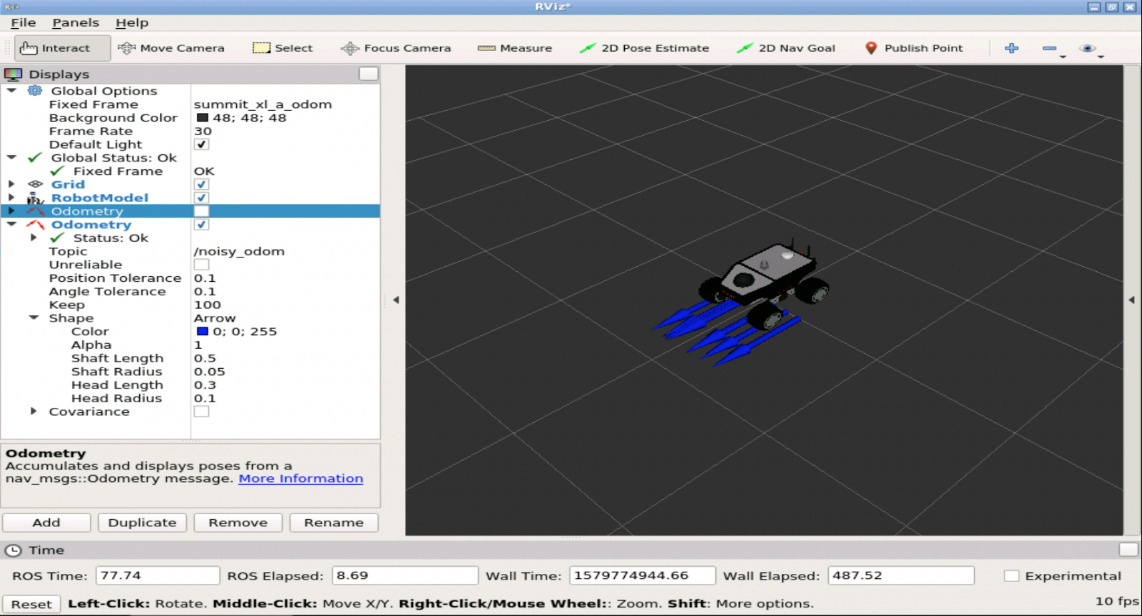
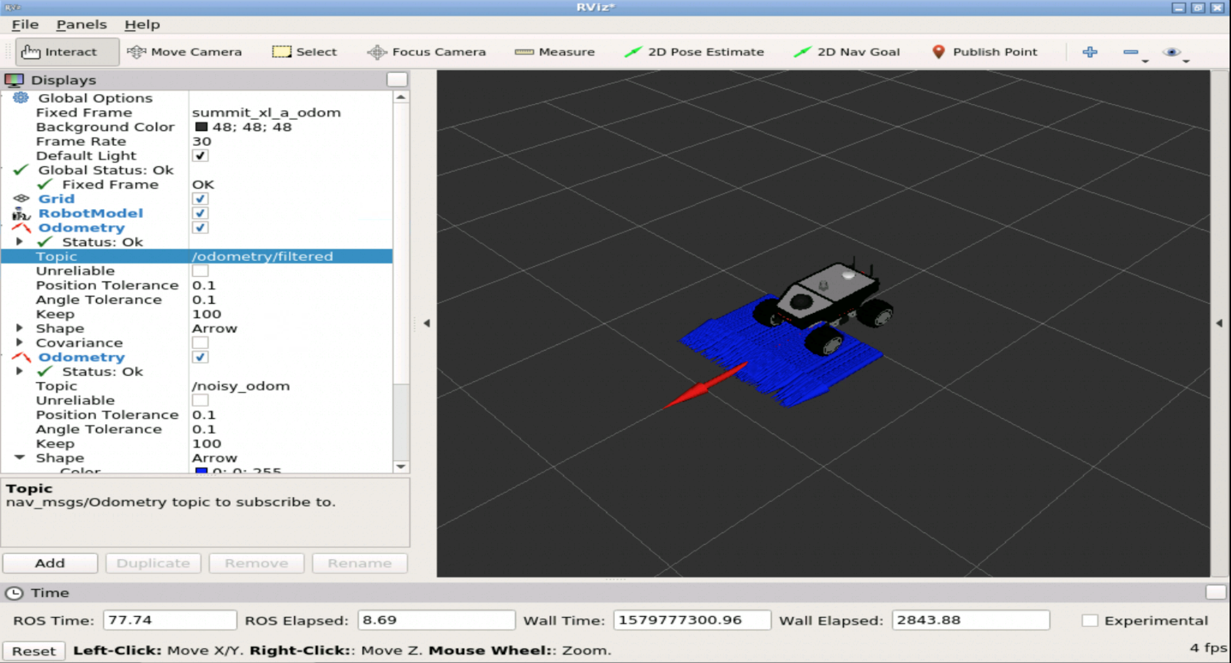
As we can see in the launch file, it spawns the robot and opens RViz (Robot Visualization). You can see RViz by opening the Graphical Tools (Tools -> Graphical Tools).
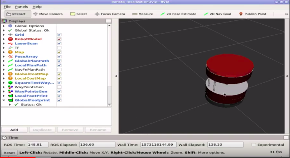
Barista robot in RViz, in ROSDS
Where is the Barista robot defined
If you look at the launch file mentioned earlier, you can see that we use the put_robot_in_world.launch file to spawn the robot. The content of the file is:
<launch>
  <arg name="base" default="barista"/>
  <arg name="stacks" default="hexagons"/>
  <arg name="3d_sensor" default="asus_xtion_pro"/>

  <arg name="x" default="0"/>
  <arg name="y" default="0"/>
  <arg name="z" default="0.5"/>
  <arg name="roll" default="0"/>
  <arg name="pitch" default="0"/>
  <arg name="yaw" default="0" />

  <arg name="urdf_file" default="$(find xacro)/xacro.py '$(find barista_description)/urdf/barista/$(arg base)_$(arg stacks)_$(arg 3d_sensor).urdf.xacro'" />
  <param name="robot_description" command="$(arg urdf_file)" />

  <node pkg="robot_state_publisher" type="robot_state_publisher" name="robot_state_publisher">
    <param name="publish_frequency" type="double" value="30.0" />
  </node>

  <!-- Gazebo model spawner -->
  <node name="spawn_$(arg base)_model" pkg="gazebo_ros" type="spawn_model"
        args="-urdf -param robot_description -model $(arg base) -x $(arg x) -y $(arg y) -z $(arg z) -R $(arg roll) -P $(arg pitch) -Y $(arg yaw)"/>

  <!-- Diagnostics publication to simulate the kobuki mobile base -->
  <node name="sim_diagnostics_pub_node" pkg="barista_gazebo" type="sim_diagnostics_pub.py"
        respawn="false" output="screen">
  </node>
  <!-- Bumper/cliff to pointcloud (not working, as it needs sensors/core messages) -->
  <!-- include file="$(find turtlebot_bringup)/launch/includes/kobuki/bumper2pc.launch.xml"/-->
</launch>
We are not going to explain this file in detail because it will take us a long time. If you need further understanding of URDF files, we highly recommend the URDF for Robot Modeling course on Robot Ignite Academy.
In this file, we essentially load the barista_hexagons_asus_xtion_pro.urdf.xacro file located on the ~/simulation_ws/src/barista/barista_description/urdf/barista/ folder.
At the end of that file we can see that we basically spawn the robot and load the sensors:
<?xml version="1.0"?>
<!--
    - Base      : barista
    - Stacks    : hexagons
    - 3d Sensor : laser-hokuyo
-->
<robot name="barista" xmlns:xacro="http://ros.org/wiki/xacro">

  <xacro:include filename="$(find turtlebot_description)/urdf/common_properties.urdf.xacro"/>
  <xacro:include filename="$(find turtlebot_description)/urdf/turtlebot_properties.urdf.xacro"/>
  <!-- Bases -->
  <xacro:include filename="$(find barista_description)/urdf/barista/barista_kobuki.urdf.xacro" />
  <!-- Stacks -->
  <xacro:include filename="$(find barista_description)/urdf/barista/barista_hexagons.urdf.xacro"/>
  <!-- 3D Sensors -->
  <!-- Barista Mods -->
  <xacro:include filename="$(find barista_description)/urdf/barista/barista_mod.urdf.xacro" />
  <xacro:include filename="$(find barista_description)/urdf/barista/barista_hokuyo.urdf.xacro" />

  <!-- Load Sensor and Common Macros and properties -->
  <xacro:include filename="$(find barista_description)/urdf/barista/macros.xacro" />
  <xacro:include filename="$(find barista_description)/urdf/barista/properties.xacro" />
  <xacro:include filename="$(find barista_description)/urdf/barista/materials.xacro" />
  <xacro:include filename="$(find barista_description)/urdf/barista/barista_loadsensor.xacro" />

  <barista_kobuki/>
  <stack_hexagons parent="base_link"/>
  <barista_mod  bottom_parent="plate_middle_link" top_parent="plate_top_link"/>
  <barista_hokuyo  parent="plate_middle_link" x_hok="0.116647" y_hok="0.0" z_hok="0.045"/>

  <barista_loadsensor  parent="barista_top_link"
                       x_loadsensor="0.014395"
                       y_loadsensor="0.0"
                       z_loadsensor="${0.082804+(loadsensor_height/2.0)}"
                       r="${loadsensor_radius}"
                       l="${loadsensor_height}"
                       mass="${loadsensor_mass}"/>

</robot>
The barista_loadsensor macro is defined in the barista_loadsensor.xacro.xacro file of the barista_description package, and has the following content:
<?xml version="1.0" ?>
<!--
  This is the load sensor used for detecting elements positioned ontop
 -->
<robot name="loadsensor" xmlns:xacro="http://ros.org/wiki/xacro">


  <xacro:macro name="barista_loadsensor" params="parent x_loadsensor y_loadsensor z_loadsensor r l mass">

    <link name="loadsensor_link">
	    <inertial>
		    <mass value="${mass}"/>
		    <origin xyz="0 0 0" rpy="0 0 0"/>
		    <cylinder_inertia mass="${mass}" r="${r}" l="${l}" />
	    </inertial>
	    <collision>
		    <origin xyz="0 0 0" rpy="0 0 0"/>
		    <geometry>
			    <cylinder length="${l}" radius="${r}"/>
		    </geometry>
	    </collision>
	    <visual>
		    <origin xyz="0 0 0" rpy="0 0 0"/>
		    <geometry>
			    <cylinder length="${l}" radius="${r}"/>
		    </geometry>
			<material name="red"/>
	    </visual>
    </link>

    <joint name="loadsensor_joint" type="fixed">
    	<origin xyz="${x_loadsensor} ${y_loadsensor} ${z_loadsensor}" rpy="0 0 0"/>
    	<parent link="${parent}"/>
    	<child link="loadsensor_link"/>
    </joint>


    <gazebo reference="loadsensor_link">
      <mu1 value="2000.0"/>
      <mu2 value="1000.0"/>
      <kp value="${kp}" />
      <kd value="${kd}" />
		<material>Gazebo/Red</material>
      <sensor name="loadsensor_link_contactsensor_sensor" type="contact">
        <always_on>true</always_on>
        <contact>
          <collision>base_footprint_fixed_joint_lump__loadsensor_link_collision_10</collision>
        </contact>
        <plugin name="loadsensor_link_plugin" filename="libgazebo_ros_bumper.so">
          <bumperTopicName>loadsensor_link_contactsensor_state</bumperTopicName>
          <frameName>loadsensor_link</frameName>
        </plugin>
      </sensor>
  	</gazebo>
  </xacro:macro>


</robot>
An important part of this file is the section that contains:
<plugin name="loadsensor_link_plugin" filename="libgazebo_ros_bumper.so">
          <bumperTopicName>loadsensor_link_contactsensor_state</bumperTopicName>
          <frameName>loadsensor_link</frameName>
        </plugin>
The plugin libgazebo_ros_bumper.so configures everything that has to do with the collisions of the load sensor.
You can see that it sets the topic /loadsensor_link_contactsensor_state to publish the data related to the load sensor.
You can see the data being published with:
rostopic echo /loadsensor_link_contactsensor_state
You can see that this topic alone publishes too much data.
Since we have to show data in the web app that we are going to create, we use the /diagnostics topic to simulate some elements, like the battery, for example, in the format that the real robot uses.
Showing the Battery status
In the barista_gazebo package, we created the sim_pick_go_return_demo.launch file. There you can see that we spawn the battery_charge_pub.py file, which basically subscribes to the /diagnostics topic and publishes into the /battery_charge topic just basic info about the battery status.
Let’s launch that file to launch the main systems:
roslaunch barista_gazebo sim_pick_go_return_demo.launch
If you open a new shell, and type the command below, you should get the battery load:
rostopic echo /battery_charge
Bear in mind that in this case, the value is simulated, given that we are still not using a real robot.
In order to test that the load_sensor works, It will be easier if you check the video https://youtu.be/Uv9yF5zifz4?t=1348 that we created.
ROS Navigation
If you look at the file sim_pick_go_return_demo.launch we mentioned earlier, in that file we are launching the navigation system, more specifically on the sections shown below:
<!-- Start the navigation systems -->
  <include file="$(find costa_robot)/launch/localization_demo.launch">
    <arg name="map_name" value="simple10x10"/>
    <arg name="real_barista" value="false"/>
  </include>
and
 <!-- We start the waypoint generator to be able to reset tables on the fly -->
  <node pkg="ros_waypoint_generator"
          type="ros_waypoint_generator"
          name="ros_waypoint_generator_node">
    </node>
To start creating the map, please consider reloading the simulation (Simulations -> Change Simulation -> Choose Launch file -> main_simple.launch).
The files related to mapping can be found on the costa_robot package. There you can find the following files:
- gmapping_demo.launch
- localization_demo.launch
- save_map.launch
- start_mapserver.launch
To create a map, after making sure the simulation is already running, we run the following:
roslaunch costa_robot gmapping_demo.launch
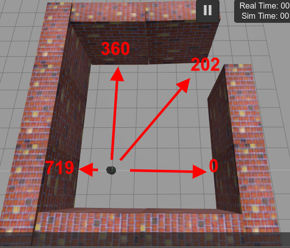
Now we have the lasers so that we can create the map. To see the lasers, please check RViz using Tools -> Graphical Tools.
You can now move the robot around by running the command below in a new shell (Tools -> Shell), to generate the map:
roslaunch turtlebot_teleop sim_keyboard_teleop.launch
While we are moving around, the map is being generated.
Then, to save the generated map, we run:
roslaunch costa_robot save_map.launch map_name:="new_map"
The new map should have been generated at ~/simulation_ws/src/barista/costa_robot/map/generated/new_map.pgm.
Now that we have the map, let’s generate the Waypoints. For that, we first launch the localization using the generated map.
roslaunch costa_robot localization_demo.launch map_name:="new_map" real_barista:="false"
Now we generate the waypoints:
roslaunch barista_gazebo start_save_waypoints_system.launch map_name:="new_map" real_barista:="false"
In order to save the waypoints, in RViz we click Publish Point and click where the robot is, then we run:
rosservice call /waypoints_save_server "name: 'HOME'"
This saves the current location of the robot as HOME. We can now move the robot around and save the new location. To move the robot around, remember that we use:
roslaunch turtlebot_teleop sim_keyboard_teleop.launch
Now we click Publish Point in RViz again and click where the robot is located and save the waypoints as Table1, for example:
rosservice call /waypoints_save_server "name: 'TABLE1'"
Great, so far we know how to start the map, start the localization and save the waypoints.
Youtube video
It may happen that you couldn’t reproduce some of the steps mentioned here. If this is the case, remember that we have the live version of this post on YouTube. Also, if you liked the content, please consider subscribing to our youtube channel. We are publishing new content ~every day.
Keep pushing your ROS Learning.