This project is about using a Two Wheeled Mobile Robot to explore features and tools provided by ROS (Robot Operating System). We start building the robot from the scratch, using URDF (Unified Robot Description Format) and RViz to visualize it. Further, we describe the inertia and show how to simplify the URDF using XACROS. Later, motion planning algorithms, such as Obstacle Avoidance and Bugs 0, 1 and 2 are developed to be used in the built robot. Some ROS packages, like robot_localization, are used to built a map and localize on it.
- Part 1: Explore the basics of robot modeling using the URDF
- Part 2: Explore the macros for URDF files using XACRO files
- Part 3: Insert a laser scan sensor to the robot
- Part 4: Read the values of the laser scanner
- Part 5: An obstacle avoidance algorithm
- Part 6: Create an algorithm to go from a point to another
- Part 7: Work with wall following robot algorithm
- Part 8: Work with the Bug 0 algorithm
- Part 9: See the Bug 0 Foil
- Part 10: Perform the motion planning task Bug 1
- Part 11: From ROS Indigo to Kinetic
- Part 12: Implement code for Bug 2 behavior
- Part 13: Use ROS GMapping in our 2 wheeled robot
Exploring ROS with a 2 Wheeled Robot #Part 1
In this video, we are going to explore the basics of robot modeling using the Unified Robot Description Format (URDF). At the end of this video, we will have a model ready and running in Gazebo simulator.
Steps to create the project as shown in the video
Step 1.1
- Head to ROS Development Studio and create a new project.
- Provide a suitable project name and some useful description.
- Open the project (this will take few seconds)
- Once the project is loaded run the IDE from the tools menu. Also verify that the inital directory structure should look like following:
.
├────── ai_ws
├────── catkin_ws
│     ├─── build
│     ├─── devel
│     └───
├────── notebook_ws
│     ├─── default.ipynb
│     └─── images
└────── simulation_ws
      ├─── build
      ├─── devel
      └─── src
The directory simulation_ws is also called simulation workspace, it is supposed to contain the code and scripts relevant for simulation. For all other files we have the catkin_ws (or catkin workspace). A few more terminologies to familiarize are xacro and macro, basically xacro is a file format encoded in xml. xacro files come with extra features called macros (akin functions) that helps in reducing the amount of written text in writing robot description. Robot model description for Gazebo simulation is described in URDF model format and xacro files simplify the process of writing elaborate robot description.
Step 1.2
Now we will create a catkin package with name m2wr_description. We will add rospy as dependency.
Start a SHELL from tools menu and navigate to ~simulation_ws/src directory as follows
$ cd simulation_ws/src
To create catkin package use teh following command
$ catkin_create_pkg m2wr_description rospy
At this point we should have the following directory structure
.
├────── ai_ws
├────── catkin_ws
│     ├─── build
│     ├─── devel
│     └───
├────── notebook_ws
│     ├─── default.ipynb
│     └─── images
└────── simulation_ws
      ├─── build
      ├─── devel
      └─── src
         ├──── CMakeLists.txt
         └──── m2wr_description
             ├─── CMakeLists.txt
             └─── package.xml
Create a directory named urdf inside m2wr_description directory. Create a file named m2wr.xacro inside the newly created urdf directory. Creating files and directories is easier (right mouse click and select appropriate option) using the IDE from the Tools menu option.
We will populate the xacro file with the following content
<?xml version="1.0" ?>

<robot name="m2wr" xmlns:xacro="https://www.ros.org/wiki/xacro" >

  <material name="black">
    <color rgba="0.0 0.0 0.0 1.0"/>
  </material>
  <material name="blue">
    <color rgba="0.203125 0.23828125 0.28515625 1.0"/>
  </material>
  <material name="green">
    <color rgba="0.0 0.8 0.0 1.0"/>
  </material>
  <material name="grey">
    <color rgba="0.2 0.2 0.2 1.0"/>
  </material>
  <material name="orange">
    <color rgba="1.0 0.423529411765 0.0392156862745 1.0"/>
  </material>
  <material name="brown">
    <color rgba="0.870588235294 0.811764705882 0.764705882353 1.0"/>
  </material>
  <material name="red">
    <color rgba="0.80078125 0.12890625 0.1328125 1.0"/>
  </material>
  <material name="white">
    <color rgba="1.0 1.0 1.0 1.0"/>
  </material>

  <gazebo reference="link_chassis">
    <material>Gazebo/Orange</material>
  </gazebo>
  <gazebo reference="link_left_wheel">
    <material>Gazebo/Blue</material>
  </gazebo>
  <gazebo reference="link_right_wheel">
    <material>Gazebo/Blue</material>
  </gazebo>

  <link name="link_chassis">
    <!-- pose and inertial -->
    <pose>0 0 0.1 0 0 0</pose>

    <inertial>
      <mass value="5"/>
      <origin rpy="0 0 0" xyz="0 0 0.1"/>
      <inertia ixx="0.0395416666667" ixy="0" ixz="0" iyy="0.106208333333" iyz="0" izz="0.106208333333"/>
    </inertial>

    <collision name="collision_chassis">
      <geometry>
        <box size="0.5 0.3 0.07"/>
      </geometry>
    </collision>

    <visual>
      <origin rpy="0 0 0" xyz="0 0 0"/>
      <geometry>
        <box size="0.5 0.3 0.07"/>
      </geometry>
      <material name="blue"/>
    </visual>

    <!-- caster front -->
    <collision name="caster_front_collision">
      <origin rpy=" 0 0 0" xyz="0.35 0 -0.05"/>
      <geometry>
        <sphere radius="0.05"/>
      </geometry>
      <surface>
        <friction>
          <ode>
            <mu>0</mu>
            <mu2>0</mu2>
            <slip1>1.0</slip1>
            <slip2>1.0</slip2>
          </ode>
        </friction>
      </surface>
    </collision>
    <visual name="caster_front_visual">
      <origin rpy=" 0 0 0" xyz="0.2 0 -0.05"/>
      <geometry>
        <sphere radius="0.05"/>
      </geometry>
    </visual>
    </link>

  <!-- Create wheel right -->

  <link name="link_right_wheel">
    <inertial>
      <mass value="0.2"/>
      <origin rpy="0 1.5707 1.5707" xyz="0 0 0"/>
      <inertia ixx="0.00052666666" ixy="0" ixz="0" iyy="0.00052666666" iyz="0" izz="0.001"/>
    </inertial>

    <collision name="link_right_wheel_collision">
      <origin rpy="0 1.5707 1.5707" xyz="0 0 0" />
      <geometry>
        <cylinder length="0.04" radius="0.1"/>
      </geometry>
    </collision>

    <visual name="link_right_wheel_visual">
      <origin rpy="0 1.5707 1.5707" xyz="0 0 0"/>
      <geometry>
        <cylinder length="0.04" radius="0.1"/>
      </geometry>
    </visual>

  </link>

  <!--   Joint for right wheel  -->
  <joint name="joint_right_wheel" type="continuous">
    <origin rpy="0 0 0" xyz="-0.05 0.15 0"/>
    <child link="link_right_wheel" />
    <parent link="link_chassis"/>
    <axis rpy="0 0 0" xyz="0 1 0"/>
    <limit effort="10000" velocity="1000"/>
    <joint_properties damping="1.0" friction="1.0" />
  </joint>

  <!-- Left Wheel link -->

  <link name="link_left_wheel">
    <inertial>
      <mass value="0.2"/>
      <origin rpy="0 1.5707 1.5707" xyz="0 0 0"/>
      <inertia ixx="0.00052666666" ixy="0" ixz="0" iyy="0.00052666666" iyz="0" izz="0.001"/>
    </inertial>

    <collision name="link_left_wheel_collision">
      <origin rpy="0 1.5707 1.5707" xyz="0 0 0" />
      <geometry>
        <cylinder length="0.04" radius="0.1"/>
      </geometry>
    </collision>

    <visual name="link_left_wheel_visual">
      <origin rpy="0 1.5707 1.5707" xyz="0 0 0"/>
      <geometry>
        <cylinder length="0.04" radius="0.1"/>
      </geometry>
    </visual>

  </link>

  <!--   Joint for right wheel  -->
  <joint name="joint_left_wheel" type="continuous">
    <origin rpy="0 0 0" xyz="-0.05 -0.15 0"/>
    <child link="link_left_wheel" />
    <parent link="link_chassis"/>
    <axis rpy="0 0 0" xyz="0 1 0"/>
    <limit effort="10000" velocity="1000"/>
    <joint_properties damping="1.0" friction="1.0" />
  </joint>

</robot>
In this xacro file we have defined the following:
- chasis + caster wheel :
linktype element - wheels :
linktype elements (left + right) - joints :
jointtype elements (left + right)
All of these elements have some common properties like inertial, collision and visual. The inertial and collision properties enable physics simulation and the visual property controls the appearance of the robot.
The joints help in defining the relative motion between links such as the motion of wheel with respect to the chassis. The wheels are links of cylindrical geometry, they are oriented (using rpy property) such that rolling is possible. The placement is controlled via the xyz property. For joints, we have specified the values for damping and friction as well. Now we can visualize the robot with rviz.
Step 1.3
To visualize the robot we just defined, we will create a lunch file named rviz.launch inside launch folder. We will populate it with following content:
<?xml version="1.0"?>
<launch>

  <param name="robot_description" command="cat '$(find m2wr_description)/urdf/m2wr.xacro'"/>

  <!-- send fake joint values -->
  <node name="joint_state_publisher" pkg="joint_state_publisher" type="joint_state_publisher">
    <param name="use_gui" value="False"/>
  </node>

  <!-- Combine joint values -->
  <node name="robot_state_publisher" pkg="robot_state_publisher" type="state_publisher"/>

  <!-- Show in Rviz   -->
  <node name="rviz" pkg="rviz" type="rviz" />

</launch>
To launch the project use the following command
$ roslaunch m2wr_description rviz.launch
Once the node is launched we need to open Graphical Tools from the Tools menu, it will help us to see the rviz window.
Once the rviz window loads, do the following:
- Change the frame to
link_chasisin Fixed Frame option - Add a Robot Description display
Step 1.4
We are now ready to simulate the robot in gazebo. We will load a empty world from the Simulations menu option
To load our robot into the empty world we will need another launch file. We will create another launch file with name spawn.launch inside the launch directory with the following contents:
<?xml version="1.0" encoding="UTF-8"?>
<launch>
    <param name="robot_description" command="cat '$(find m2wr_description)/urdf/m2wr.xacro'" />

    <arg name="x" default="0"/>
    <arg name="y" default="0"/>
    <arg name="z" default="0.5"/>

    <node name="mybot_spawn" pkg="gazebo_ros" type="spawn_model" output="screen"
          args="-urdf -param robot_description -model m2wr -x $(arg x) -y $(arg y) -z $(arg z)" />

</launch>
Next we will spawn our robot with the launch file in the empty gazebo world. Use the following command
$ roslaunch m2wr_description spawn.launch
The robot should load in the gazebo window
At this point our directory structure should look like following
.
├────── ai_ws
├────── catkin_ws
│     ├─── build
│     ├─── devel
│     └───
├────── notebook_ws
│     ├─── default.ipynb
│     └─── images
└────── simulation_ws
      ├─── build
      ├─── devel
      └─── src
         ├── CMakeLists.txt
         └── m2wr_description
            ├── CMakeLists.txt
            ├── launch
            │   ├── rviz.launch
            │   └── spawn.launch
            ├── package.xml
            └── urdf
                └── m2wr.xacro
Step 1.5
Now we are ready to add control to our robot. We will add a new element called plugin to our xacro file. We will add a differential drive plugin to our robot. The new tag looks like follows:
<gazebo>
    <plugin filename="libgazebo_ros_diff_drive.so" name="differential_drive_controller">
      <alwaysOn>true</alwaysOn>
      <updateRate>20</updateRate>
      <leftJoint>joint_left_wheel</leftJoint>
      <rightJoint>joint_right_wheel</rightJoint>
      <wheelSeparation>0.4</wheelSeparation>
      <wheelDiameter>0.2</wheelDiameter>
      <torque>0.1</torque>
      <commandTopic>cmd_vel</commandTopic>
      <odometryTopic>odom</odometryTopic>
      <odometryFrame>odom</odometryFrame>
      <robotBaseFrame>link_chassis</robotBaseFrame>
    </plugin>
  </gazebo>
Add this element inside the <robot> </robot> tag and relaunch the project. Now we will be able to control the robot, we can check this by listing the available topics using following command
$ rostopic list
To control the motion of the robot we can use the keyboard_teleop to publish motion commands using the keyboard. Use the following command in Shell
$ rosrun teleop_twist_keyboard teleop_twist_keyboard.py
Now we can make the robot navigate with keyboard keys. This finishes the part-1.
References
RDS: https://rds.theconstructsim.com/
Source Code Repository: https://bitbucket.org/theconstructcore/two-wheeled-robot/
Inertia Matrix reference: https://en.wikipedia.org/wiki/List_of_moments_of_inertia
[irp posts=”7150″ name=”ROS Q&A | Showing my own URDF model in Gazebo”]
Exploring ROS with a 2 Wheeled Robot #Part 2 – URDF Macros
In this video, we are going to explore the macros for URDF files, using XACRO files. At the end of this video, we will have the same model organized in different files, in a organized way.
Steps continued from last part
Step 2.1
In the last 5 steps we acheived the following:
- Created a
xacrofile that contains the urdf description of our robot - Created a
launchfiles to spawn the robot in gazebo environment - Controlled the simulated robot using keyboard teleoperation
In this part we will organize the existing project to make it more readable and modular. Even though our robot description had only few components, we had written a lengthy xacro file. Also in robot spawn launch file we have used the following line
<param name="robot_description" command="cat '$(find m2wr_description)/urdf/m2wr.xacro'" />
Here we are using the cat command to read the contents of m2wr.xacro file into robot_description parameter. However, to use the features of the xacro file we need to parse and execute the xacro file and to achieve that we will modify the above line to
<param name="robot_description" command="$(find xacro)/xacro.py '$(find m2wr_description)/urdf/m2wr.xacro'" />
The above command, uses the xacro.py file to exucute the instructions of m2wr.xacro file. A similar edit is needed for the rviz.launch file as well. So change the following line in rviz.launch file
<param name="robot_description" command="cat '$(find m2wr_description)/urdf/m2wr.xacro'" />
to
<param name="robot_description" command="$(find xacro)/xacro.py '$(find m2wr_description)/urdf/m2wr.xacro'"/>
Step 2.2
At the moment, our xacro file does not contain any instructions. We will now split up the large m2wr.xacro file into smaller files and using the features of xacro we will assimilate the smaller files.
First we will extract the material properties from our xacro file and place them in a new file called materials.xacro. We will create a new file named materials.xacro inside the urdf folder and write the following contents into it
<?xml version="1.0" ?>
<robot name="m2wr" xmlns:xacro="https://www.ros.org/wiki/xacro" >
  <material name="black">
    <color rgba="0.0 0.0 0.0 1.0"/>
  </material>
  <material name="blue">
    <color rgba="0.203125 0.23828125 0.28515625 1.0"/>
  </material>
  <material name="green">
    <color rgba="0.0 0.8 0.0 1.0"/>
  </material>
  <material name="grey">
    <color rgba="0.2 0.2 0.2 1.0"/>
  </material>
  <material name="orange">
    <color rgba="1.0 0.423529411765 0.0392156862745 1.0"/>
  </material>
  <material name="brown">
    <color rgba="0.870588235294 0.811764705882 0.764705882353 1.0"/>
  </material>
  <material name="red">
    <color rgba="0.80078125 0.12890625 0.1328125 1.0"/>
  </material>
  <material name="white">
    <color rgba="1.0 1.0 1.0 1.0"/>
  </material>
</robot>
We need to replace all material elements in the original m2wr.xacro file with following include directive
<xacro:include filename="$(find m2wr_description)/urdf/materials.xacro" />
To test the changes we can start the rviz visualization with command
$ roslaunch m2wr_description rviz.launch
Use Graphical Tool to see the rviz output
Going further we will now remove more code from the m2wr.xacro file and place it in a new file. Create a new file with name m2wr.gazebo inside the urdf directory. We will move all the gazebo tags from the m2wr.xacro file to this new file. We will need to add the enclosing
<?xml version="1.0" ?>
<robot name="m2wr" xmlns:xacro="https://www.ros.org/wiki/xacro" >
<gazebo reference="link_chassis">
    <material>Gazebo/Orange</material>
  </gazebo>
  <gazebo reference="link_left_wheel">
    <material>Gazebo/Blue</material>
  </gazebo>
  <gazebo reference="link_right_wheel">
    <material>Gazebo/Blue</material>
  </gazebo>

  <gazebo>
    <plugin filename="libgazebo_ros_diff_drive.so" name="differential_drive_controller">
      <alwaysOn>true</alwaysOn>
      <updateRate>20</updateRate>
      <leftJoint>joint_left_wheel</leftJoint>
      <rightJoint>joint_right_wheel</rightJoint>
      <wheelSeparation>0.4</wheelSeparation>
      <wheelDiameter>0.2</wheelDiameter>
      <torque>0.1</torque>
      <commandTopic>cmd_vel</commandTopic>
      <odometryTopic>odom</odometryTopic>
      <odometryFrame>odom</odometryFrame>
      <robotBaseFrame>link_chassis</robotBaseFrame>
    </plugin>
  </gazebo>
We will add another include directive to the m2wr.xacro file (as shown)
<xacro:include filename="$(find m2wr_description)/urdf/gazebo.xacro" />
To see whether everything works, we can launch the gazebo simulation of and empty world and spawn the robot. First we will start the gazebo simulation from the Simulations menu option and then spawn a robot with the following command
$ roslaunch m2wr_description spawn.launch
We should see the robot being spawned
Step 2.3
Next we will use macros, which are like functions, to reduce the remaining code in m2wr.xacro file.
Create a new file macro.xacro inside the urdf directory with following contents
<?xml version="1.0"?>
<robot xmlns:xacro="http://www.ros.org/wiki/xacro">
    <xacro:macro name="link_wheel" params="name">
        <link name="${name}">
            <inertial>
              <mass value="0.2"/>
              <origin rpy="0 1.5707 1.5707" xyz="0 0 0"/>
              <inertia ixx="0.000526666666667" ixy="0" ixz="0" iyy="0.000526666666667" iyz="0" izz="0.001"/>
            </inertial>
            <collision name="link_right_wheel_collision">
              <origin rpy="0 1.5707 1.5707" xyz="0 0 0"/>
              <geometry>
                <cylinder length="0.04" radius="0.1"/>
              </geometry>
            </collision>
            <visual name="${name}_visual">
              <origin rpy="0 1.5707 1.5707" xyz="0 0 0"/>
              <geometry>
                <cylinder length="0.04" radius="0.1"/>
              </geometry>
            </visual>
        </link>
    </xacro:macro>

    <xacro:macro name="joint_wheel" params="name child origin_xyz">
      <joint name="${name}" type="continuous">
        <origin rpy="0 0 0" xyz="${origin_xyz}"/>
        <child link="${child}"/>
        <parent link="link_chassis"/>
        <axis rpy="0 0 0" xyz="0 1 0"/>
        <limit effort="10000" velocity="1000"/>
        <joint_properties damping="1.0" friction="1.0"/>
      </joint>
    </xacro:macro>

</robot>
In the above code we have defined three macros, their purpose is to take parameters and create the required element (`link` element). The first macro is named link_wheel and it accepts only one parameter name. It creates a wheel link with the name passed in the parameter. The second macro accepts three parameters name, child and origin_xyz and it creates a joint link.
We will use these macro in our robot description file (m2wr.xacro). To use macros we will replace the link element by the macros as follows
<link name="link_right_wheel">
    <inertial>
      <mass value="0.2"/>
      <origin rpy="0 1.5707 1.5707" xyz="0 0 0"/>
      <inertia ixx="0.00052666666" ixy="0" ixz="0" iyy="0.00052666666" iyz="0" izz="0.001"/>
    </inertial>

    <collision name="link_right_wheel_collision">
      <origin rpy="0 1.5707 1.5707" xyz="0 0 0" />
      <geometry>
        <cylinder length="0.04" radius="0.1"/>
      </geometry>
    </collision>

    <visual name="link_right_wheel_visual">
      <origin rpy="0 1.5707 1.5707" xyz="0 0 0"/>
      <geometry>
        <cylinder length="0.04" radius="0.1"/>
      </geometry>
    </visual>
 </link>

 <link name="link_left_wheel">
    <inertial>
      <mass value="0.2"/>
      <origin rpy="0 1.5707 1.5707" xyz="0 0 0"/>
      <inertia ixx="0.00052666666" ixy="0" ixz="0" iyy="0.00052666666" iyz="0" izz="0.001"/>
    </inertial>

    <collision name="link_left_wheel_collision">
      <origin rpy="0 1.5707 1.5707" xyz="0 0 0" />
      <geometry>
        <cylinder length="0.04" radius="0.1"/>
      </geometry>
    </collision>

    <visual name="link_left_wheel_visual">
      <origin rpy="0 1.5707 1.5707" xyz="0 0 0"/>
      <geometry>
        <cylinder length="0.04" radius="0.1"/>
      </geometry>
    </visual>
 </link>
replaced by
<xacro:link_wheel name="link_right_wheel" />
<xacro:link_wheel name="link_left_wheel" />
Similar addition for the link_left_wheel. We will also replace the two wheel joint elements with following
<xacro:joint_wheel name="joint_right_wheel"  child="link_right_wheel"  origin_xyz="-0.05 0.15 0"  />
<xacro:joint_wheel name="joint_left_wheel"   child="link_left_wheel"   origin_xyz="-0.05 -0.15 0"  />
We also need to add the include directive for the macro.xacro file (in m2wr.xacro file)
<xacro:include filename="$(find m2wr_description)/urdf/macro.xacro" />
The final contents of the m2wr.xacro shoud be following
<?xml version="1.0" ?>
<robot name="m2wr" xmlns:xacro="https://www.ros.org/wiki/xacro" >

  <!-- include the xacro files-->
  <xacro:include filename="$(find m2wr_description)/urdf/materials.xacro" />
  <xacro:include filename="$(find m2wr_description)/urdf/m2wr.gazebo" />
  <xacro:include filename="$(find m2wr_description)/urdf/macro.xacro" />

  <!-- Chasis defined here -->
  <link name="link_chassis">
    <pose>0 0 0.1 0 0 0</pose>
    <inertial>
      <mass value="5"/>
      <origin rpy="0 0 0" xyz="0 0 0.1"/>
      <inertia ixx="0.0395416666667" ixy="0" ixz="0" iyy="0.106208333333" iyz="0" izz="0.106208333333"/>
    </inertial>

    <collision name="collision_chassis">
      <geometry>
        <box size="0.5 0.3 0.07"/>
      </geometry>
    </collision>

    <visual>
      <origin rpy="0 0 0" xyz="0 0 0"/>
      <geometry>
        <box size="0.5 0.3 0.07"/>
      </geometry>
      <material name="blue"/>
    </visual>

    <!-- caster front -->
    <collision name="caster_front_collision">
      <origin rpy=" 0 0 0" xyz="0.35 0 -0.05"/>
      <geometry>
        <sphere radius="0.05"/>
      </geometry>
      <surface>
        <friction>
          <ode>
            <mu>0</mu>
            <mu2>0</mu2>
            <slip1>1.0</slip1>
            <slip2>1.0</slip2>
          </ode>
        </friction>
      </surface>
    </collision>
    <visual name="caster_front_visual">
      <origin rpy=" 0 0 0" xyz="0.2 0 -0.05"/>
      <geometry>
        <sphere radius="0.05"/>
      </geometry>
    </visual>
    </link>


  <!-- Create wheel right -->

   <xacro:link_wheel name="link_right_wheel" />
   <xacro:joint_wheel name="joint_right_wheel"  child="link_right_wheel"  origin_xyz="-0.05 0.15 0"  />


  <!-- Left Wheel link -->

  <xacro:link_wheel name="link_left_wheel" />
  <xacro:joint_wheel name="joint_left_wheel"   child="link_left_wheel"   origin_xyz="-0.05 -0.15 0"  />

</robot>
The above code is much shorter than what we started with. We have only used a few of the features available in `xacro` description.
Finally, we can test everything together by launching the gazebo simulator and spawing our robot. Start a new gazebo simulator with empty world and spawn our robot
$ roslaunch m2wr_description spawn.launch
That is it, we have optimized our code by splitting the large xacro file into other files and using macros.
References
RDS: https://rds.theconstructsim.com/
Source Code Repository: https://bitbucket.org/theconstructcore/two-wheeled-robot
[irp posts=”9004″ name=”My Robotic Manipulator – Part #1 – Basic URDF and RViz”]
Exploring ROS with a 2 Wheeled Robot #Part 3 – URDF Laser Scan Sensor
In this video, we are going to insert a laser scan sensor to a 2 wheeled robot the robot.
Steps continued from last part
Step 3.1
Now we will add a laser scan sensor to our robots urdf model. We will modify the urdf file (m2wr.xacro) as follows
- Add a
linkelement to our robot. Thislinkwill be cylindrical in shape and will represent the sensor. - Add a
jointelement to our robot. This will connect the sensor to robot body rigidly. - Define a new
macroto calculate the inertial property of a cylinder using its dimensions (lengthandradius) - Finally a laser scan sensor
pluginelement will add sensing ability to thelinkthat we created (the cylinder representing the sensor).
Open the m2wr.xacro file and add a new link element and a new joint element
 <link name="sensor_laser">
    <inertial>
      <origin xyz="0 0 0" rpy="0 0 0" />
      <mass value="1" />
      <!-- RANDOM INERTIA BELOW -->
      <inertia ixx="0.02" ixy="0" ixz="0" iyy="0.02" iyz="0" izz="0.02"/>
    </inertial>

    <visual>
      <origin xyz="0 0 0" rpy="0 0 0" />
      <geometry>
        <cylinder radius="0.05" length="0.1"/>
      </geometry>
      <material name="white" />
    </visual>

    <collision>
      <origin xyz="0 0 0" rpy="0 0 0"/>
      <geometry>
        <cylinder radius="0.05" length="0.1"/>
      </geometry>
    </collision>
  </link>

  <joint name="joint_sensor_laser" type="fixed">
    <origin xyz="0.15 0 0.05" rpy="0 0 0"/>
    <parent link="link_chassis"/>
    <child link="sensor_laser"/>
  </joint>
The above code block will result in the following visualization
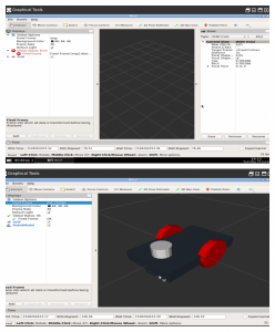
Step 3.2
The link element we just added (for acting as sensor) has random inertia property (see line 5 of the above code). We can write some sane values using a macro that will calculate the inertia values using cylinder dimensions. For this we add a new macro to our macro.xacro script. Add the following macro to the file
<xacro:macro name="cylinder_inertia" params="mass r l">
    <inertia ixx="${mass*(3*r*r+l*l)/12}" ixy = "0" ixz = "0"
                iyy="${mass*(3*r*r+l*l)/12}" iyz = "0" izz="${mass*(r*r)/2}" />
</xacro:macro>
Lets use this macro in the sensor description link by modifying the inertia tag with following
<xacro:cylinder_inertia mass="1" r="0.05" l="0.1" />
Now we can simulate the robot and see if everything works well. Load an empty world in gazebo simulator window. Also open a Shell window and run the following command
$ roslaunch m2wr_description spawn.launch
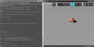 Next we need to add the sensor beharior to the
 link. To do so we will use the laser gazebo plugin. Information about this plugin is available here. Open the m2wr.gazebo file and add the following plugin element
<gazebo reference="sensor_laser">
    <sensor type="ray" name="head_hokuyo_sensor">
      <pose>0 0 0 0 0 0</pose>
      <visualize>false</visualize>
      <update_rate>20</update_rate>
      <ray>
        <scan>
          <horizontal>
            <samples>720</samples>
            <resolution>1</resolution>
            <min_angle>-1.570796</min_angle>
            <max_angle>1.570796</max_angle>
          </horizontal>
        </scan>
        <range>
          <min>0.10</min>
          <max>10.0</max>
          <resolution>0.01</resolution>
        </range>
        <noise>
          <type>gaussian</type>
          <mean>0.0</mean>
          <stddev>0.01</stddev>
        </noise>
      </ray>
      <plugin name="gazebo_ros_head_hokuyo_controller" filename="libgazebo_ros_laser.so">
        <topicName>/m2wr/laser/scan</topicName>
        <frameName>sensor_laser</frameName>
      </plugin>
    </sensor>
  </gazebo>
This code specifies many important parameters
Update rate : Controls how often (how fast) the laser data is captured
samples : Defines how how many readings are contained in one scan
resolution : Defines the minimum angular distance between readings captured in a laser scan
range : Defines the minimum sense distance and maximum sense distance. If a point is below minimum sense its reading becomes zero(0) and if a point is further than the maximum sense distance its reading becomes inf. The range resolution defines the minimum distance between 2 points such that two points can be resolved as two separate points.
noise : This parameter lets us add gaussian noise to the range data captured by the sensor
topicName : Defines the name which is used for publishing the laser data
frameName : Defines the link to which the plugin has to be applied
With this plugin incorporated in the urdf file we are now ready to simulate and visualize the laser scan in action. Start the empty world and spawn the robot by launching the spawn.launch file in a Shell. To verify the working of the scan sensor check the list of topics in Shell window with following command
$ rostopic list
You should get /m2wr/laser/scan in the list of topics
Step 3.3
We will visualize the laser scan data with rviz. First we will populate the robot environment with a few obstacles to better see the laser scan result. Use the box icon on top right of gazebo window to create a few box type obstacles (simply click and drop)
To start rviz visualization launch the rviz.launch file in a new Shell and use Graphical Tool window to load the visualization. Use the following command to launch rviz
$ roslaunch m2wr_description rviz.launch
After starting rviz open the Graphical Tools window. Once rviz window loads you need to do the following settings
- Select odom in the Fixed Frame field (see the image below)
- Add two new displays using the Add button on the left bottom of rviz screen. The first display should be RobotModel and the other should be LaserScan
- Expand the LaserScan display by double clicking on its name and choose Topic as /m2wr/laser/scan (as shown in image below)
Now when we move the robot we can see the laser scan changing.
References
RDS: https://rds.theconstructsim.com/
Source Code Repository: https://bitbucket.org/theconstructcore/two-wheeled-robot
Gazebo plugins: http://gazebosim.org/tutorials?tut=ros_gzplugins#Laser
ROS URDF Links: http://wiki.ros.org/urdf/XML/link
ROS URDF Joints: http://wiki.ros.org/urdf/XML/joint
Exploring ROS using a 2 Wheeled Robot – Part 4
In this video, we are going to read the values of the laser scanner and filter a small part to work with
Steps to recreate the project as shown in the video
Step 4.1
- Head to ROS Development Studio and create a new project. Provide a suitable project name and some useful description. (We have named the project video_no_4)
- Open the project (this will take few seconds).
- We will clone the github repository to start. Open a Shell from the Tools menu and run the following commands in the Shell
$ cd simulation_ws/src
$ git clone https://marcoarruda@bitbucket.org/theconstructcore/two-wheeled-robot-simulation.git
- We should have the following directory structure at this point
.
├────── ai_ws
├────── catkin_ws
│     ├─── build
│     ├─── devel
│     └───
├────── notebook_ws
│     ├─── default.ipynb
│     └─── images
└────── simulation_ws
      ├─── build
      ├─── devel
      └─── src
          ├── m2wr_description
          │   ├── CMakeLists.txt
          │   ├── launch
          │   ├── package.xml
          │   └── urdf
          └── my_worlds
              ├── CMakeLists.txt
              ├── launch
              ├── package.xml
              └── worlds
The package m2wr_description contains the project files developed so far (i.e. robot + laser scan sensor). The other package my_worlds contains two directories
- launch : Contains a launch file (we will use it shortly)
- worlds : Contains multiple world description files
From Simulations menu, choose the option Select launch file… and select the world1.launch option
Step 4.2
We will create a new catkin package named motion_plan with dependencies rospy, std_msgs, geometry_msgs and sensor_msgs. Open a Shell from the Tools menu and write the following commands
$ cd ~/catkin_ws/src $ catkin_create_pgk motion_plan rospy std_msgs geometry_msgs sensor_msgs $ cd motion_plan $ mkdir scripts $ touch scripts/reading_laser.py
These commands will create a directory (named scripts) inside the motion_plan package. This directory will contains a python scripts (reading_laser.py) that we will use to read the laser scan data coming on the /m2wr/laser/scan topic (we created this topic in last part). Add the following code to the reading_laser.py file
#! /usr/bin/env python

import rospy
from sensor_msgs.msg import LaserScan

def clbk_laser(msg):
    # 720/5 = 144
    regions = [
      min(msg.ranges[0:143]),
      min(msg.ranges[144:287]),
      min(msg.ranges[288:431]),
      min(msg.ranges[432:575]),
      min(msg.ranges[576:713]),
     ]
     rospy.loginfo(regions)

def main():
    rospy.init_node('reading_laser')
    sub= rospy.Subscriber("/m2wr/laser/scan", LaserScan, clbk_laser)

    rospy.spin()

if __name__ == '__main__':
    main()
We will make this script executable with following commands
$ cd ~/catkin_ws/src/motion_plan/scripts/ $ chmod +x reading_laser.py
Before we run this file, we need to spawn our robot into the gazebo simulation. Use the following commands
$ roslaunch m2wr_description spawn.launch $ rosrun motion_plan reading_laser.py
Once we have verified that everythings is working fine. We will modify the callback function to following
def clbk_laser(msg):
    # 720/5 = 144
    regions = [
      min(msg.ranges[0:143]),
      min(msg.ranges[144:287]),
      min(msg.ranges[288:431]),
      min(msg.ranges[432:575]),
      min(msg.ranges[576:713]),
     ]
     rospy.loginfo(regions)
The above code converts the 720 readings contained inside the LaserScan msg into five distinct readings. Each reading is the minimum distance measured on a sector of 60 degrees (total 5 sectors = 180 degrees).
Lets run this code again and see the data
Step 4.3
We can see the changes in range measurements as we move the robot near to the boundaries. One noticable thing is the inf value that is measured when the wall is away.
We can modify the code to change this value to read maximum range. The changed code is
def clbk_laser(msg):
    # 720/5 = 144
    regions = [
      min(min(msg.ranges[0:143]), 10),
      min(min(msg.ranges[144:287]), 10),
      min(min(msg.ranges[288:431]), 10),
      min(min(msg.ranges[432:575]), 10),
     min( min(msg.ranges[576:713]), 10),
     ]
     rospy.loginfo(regions)
With this modification we will only receive a value of range between 0 and 10.
This finishes the part 4.
References
RDS: https://rds.theconstructsim.com/
Source Code Repository: https://bitbucket.org/theconstructcore/two-wheeled-robot
Gazebo plugins: http://gazebosim.org/tutorials?tut=ros_gzplugins#Laser
Exploring ROS with a 2 Wheeled Robot – Part 5
In this video an obstacle avoidance algorithm is explained an shown how it works.
Steps to recreate the project as shown in the video
Step 5.1
- Head to ROS Development Studio and create a new project.
- Provide a suitable project name and some useful description. (We have named the project part 5-obstacle avoidance)
- Load/Start the project (this will take few seconds).
- Clone the github repository two-wheeled-robot – Simulation.
- Checkout to the right branch ( here is more information about branch and branching in git )
- Open a Shell from the Tools menu and run the following commands in the Shell
$ cd simulation_ws/src
$ git clone https://marcoarruda@bitbucket.org/theconstructcore/two-wheeled-robot-simulation.git
$ cd two-wheeled-robot-simulation
$ git checkout 16e45ce
- Compile the project to make it ready to use
cd ~/simulation_ws/src
catkin_make
- Clone another github repository two-wheeled-robot – Motion Planning. Execute the following commands in the Shell
$ cd catkin_ws/src
$ git clone https://marcoarruda@bitbucket.org/theconstructcore/two-wheeled-robot-motion-planning.git
- Compile the project to make it ready to use
cd ~/catkin_ws/src
catkin_make
- At this point we should have the following directory structure
.
├────── ai_ws
├────── catkin_ws
│     ├─── build/
│     ├─── devel/
│     └─── src
│         ├── CMakeLists.txt
│         └── two-wheeled-robot-motion-planning
│             ├── CMakeLists.txt
│             ├── examples/
│             ├── launch/
│             ├── package.xml
│             └── scripts/
├────── notebook_ws
│     ├─── default.ipynb
│     └─── images/
└────── simulation_ws
    ├─── build/
    ├─── devel/
    └─── src
        ├── m2wr_description
        │   ├── CMakeLists.txt
        │   ├── launch/
        │   ├── package.xml
        │   └── urdf/
        └── my_worlds
            ├── CMakeLists.txt
            ├── launch/
            │   └── world.launch
            ├── package.xml
            └── worlds/
                 ├── world01.world
                 └── world02.world
Step 5.2
Start a simulation using the Simulations menu option. Select the world.launch option and launch the simulation.
Now we will take a look at the obstacle avoidance algorithm. Open the IDE and browse to the file ~/catkin_ws/src/two-wheeled-robot-motion-planning/scripts/obstacle_avoidance.py. There are 3 functions defined in this file:
main
This is the entry point of the file. This function sets up a Subscriber to the laser scan topic /m2wr/laser/scan and a Publisher to /cmd_vel topic.
    def main():
        global pub

        rospy.init_node('reading_laser')
        pub = rospy.Publisher('/cmd_vel', Twist, queue_size=1)
        sub = rospy.Subscriber('/m2wr/laser/scan', LaserScan, clbk_laser)
        rospy.spin()
clbk_laser
We need to provide a callback function to the Subscriber defined in main, for this purpose we have this function. It receives laser scan data comprising of 720 readings and converts it into 5 readings (details in part 4 video).
    def clbk_laser(msg):
        regions = {
            'right':  min(min(msg.ranges[0:143]), 10),
            'fright': min(min(msg.ranges[144:287]), 10),
            'front':  min(min(msg.ranges[288:431]), 10),
            'fleft':  min(min(msg.ranges[432:575]), 10),
            'left':   min(min(msg.ranges[576:713]), 10),
        }

        take_action(regions)
take_action
This function implements the obstacle avoidance logic. Based on the distances sensed in the five region (left, center-left, center, center-right, right). We consider possible combinations for obstacles, once we identify the obstacle configuration we steer the robot away from obstacle.
def take_action(regions):
    msg = Twist()
    linear_x = 0
    angular_z = 0

    state_description = ''

    if regions['front'] > 1 and regions['fleft'] > 1 and regions['fright'] > 1:
        state_description = 'case 1 - nothing'
        linear_x = 0.6
        angular_z = 0
    elif regions['front'] < 1 and regions['fleft'] > 1 and regions['fright'] > 1:
        state_description = 'case 2 - front'
        linear_x = 0
        angular_z = 0.3
    elif regions['front'] > 1 and regions['fleft'] > 1 and regions['fright'] < 1:
        state_description = 'case 3 - fright'
        linear_x = 0
        angular_z = 0.3
    elif regions['front'] > 1 and regions['fleft'] < 1 and regions['fright'] > 1:
        state_description = 'case 4 - fleft'
        linear_x = 0
        angular_z = -0.3
    elif regions['front'] < 1 and regions['fleft'] > 1 and regions['fright'] < 1:
        state_description = 'case 5 - front and fright'
        linear_x = 0
        angular_z = 0.3
    elif regions['front'] < 1 and regions['fleft'] < 1 and regions['fright'] > 1:
        state_description = 'case 6 - front and fleft'
        linear_x = 0
        angular_z = -0.3
    elif regions['front'] < 1 and regions['fleft'] < 1 and regions['fright'] < 1:
        state_description = 'case 7 - front and fleft and fright'
        linear_x = 0
        angular_z = 0.3
    elif regions['front'] > 1 and regions['fleft'] < 1 and regions['fright'] < 1:
        state_description = 'case 8 - fleft and fright'
        linear_x = 0.3
        angular_z = 0
    else:
        state_description = 'unknown case'
        rospy.loginfo(regions)

    rospy.loginfo(state_description)
    msg.linear.x = -linear_x
    msg.angular.z = angular_z
    pub.publish(msg)
To test the logic lets run the simulation. We have the world loaded, now we will spawn the differential drive robot with following command
$ roslaunch m2wr_description spawn.launch
Finally we launch the obstacle avoidance script to move the robot around and avoid obstacles
$ rosrun motion_plan obstacle_avoidance.py
That finishes the instructions. You can change various settings like speed of robot, sensing distance etc and see how it works.
References
RDS: https://rds.theconstructsim.com
Public Repositories:
Simulation: https://bitbucket.org/theconstructcore/two-wheeled-robot-simulation
Motion Planning: https://bitbucket.org/theconstructcore/two-wheeled-robot-motion-planning
Exploring ROS with a 2 Wheeled Robot – Part 6
In this video, we are going create an algorithm to go from a point to another using the odometry data to localize the robot.
Steps to recreate the project as shown in the video (continued from part 5)
Step 6.1
In this part we are going to implement a simple navigation algorithm to move our robot from any point to a desired point. We will use the concept of state machines to implement the navigation logic. In a state machine there are finite number of states that represent the current situation (or behavior) of the system. In our case, we have three states
- Fix Heading : Denotes the state when
robot headingdiffers from thedesired headingby more than a threshold (represented byyaw_precision_in code) - Go Straight : Denotes the state when robot has correct heading but is away from the desired point by a distance greater than some threshold ( represented by
dist_precision_in code) - Done : Denotes the state when robot has correct heading and has reached the destination.
The robot can be in any one state at a time and can switch to other states as different conditions arise. This is depicted by the following state transition diagram
To implement this state logic lets create a new python script inside the ~/catkin_ws/src/two-wheeled-robot-motion-planning/scripts/ directory named go_to_point.py with following content
#! /usr/bin/env python

# import ros stuff
import rospy
from sensor_msgs.msg import LaserScan
from geometry_msgs.msg import Twist, Point
from nav_msgs.msg import Odometry
from tf import transformations

import math

# robot state variables
position_ = Point()
yaw_ = 0
# machine state
state_ = 0
# goal
desired_position_ = Point()
desired_position_.x = -3
desired_position_.y = 7
desired_position_.z = 0
# parameters
yaw_precision_ = math.pi / 90 # +/- 2 degree allowed
dist_precision_ = 0.3

# publishers
pub = None

# callbacks
def clbk_odom(msg):
    global position_
    global yaw_

    # position
    position_ = msg.pose.pose.position

    # yaw
    quaternion = (
        msg.pose.pose.orientation.x,
        msg.pose.pose.orientation.y,
        msg.pose.pose.orientation.z,
        msg.pose.pose.orientation.w)
    euler = transformations.euler_from_quaternion(quaternion)
    yaw_ = euler[2]

def change_state(state):
    global state_
    state_ = state
    print 'State changed to [%s]' % state_

def fix_yaw(des_pos):
    global yaw_, pub, yaw_precision_, state_
    desired_yaw = math.atan2(des_pos.y - position_.y, des_pos.x - position_.x)
    err_yaw = desired_yaw - yaw_

    twist_msg = Twist()
    if math.fabs(err_yaw) > yaw_precision_:
        twist_msg.angular.z = 0.7 if err_yaw > 0 else -0.7

    pub.publish(twist_msg)

    # state change conditions
    if math.fabs(err_yaw) <= yaw_precision_:
        print 'Yaw error: [%s]' % err_yaw
        change_state(1)

def go_straight_ahead(des_pos):
    global yaw_, pub, yaw_precision_, state_
    desired_yaw = math.atan2(des_pos.y - position_.y, des_pos.x - position_.x)
    err_yaw = desired_yaw - yaw_
    err_pos = math.sqrt(pow(des_pos.y - position_.y, 2) + pow(des_pos.x - position_.x, 2))

    if err_pos > dist_precision_:
        twist_msg = Twist()
        twist_msg.linear.x = 0.6
        pub.publish(twist_msg)
    else:
        print 'Position error: [%s]' % err_pos
        change_state(2)

    # state change conditions
    if math.fabs(err_yaw) > yaw_precision_:
        print 'Yaw error: [%s]' % err_yaw
        change_state(0)

def done():
    twist_msg = Twist()
    twist_msg.linear.x = 0
    twist_msg.angular.z = 0
    pub.publish(twist_msg)

def main():
    global pub

    rospy.init_node('go_to_point')

    pub = rospy.Publisher('/cmd_vel', Twist, queue_size=1)

    sub_odom = rospy.Subscriber('/odom', Odometry, clbk_odom)

    rate = rospy.Rate(20)
    while not rospy.is_shutdown():
        if state_ == 0:
            fix_yaw(desired_position_)
        elif state_ == 1:
            go_straight_ahead(desired_position_)
        elif state_ == 2:
            done()
            pass
        else:
            rospy.logerr('Unknown state!')
            pass
        rate.sleep()

if __name__ == '__main__':
    main()
Lets analyze the contents of this script. We have defined the following function
main
This is the entry point of the file. This function sets up a Subscriber to the odometry topic /odom and a Publisher to /cmd_vel topic to command velocity of the robot. Further this function processes the state machine depending on the value ofstatevariable.clbk_odom
This is a callback function for the Subscriber defined in main. This function receives theodometrydata and extracts the position and yaw information. Theodometrydata encodes orientation information in quaternions. To obtains yaw the quaternion is converted into euler angles (line 43)change_state
This function changes the value of the globalstatevariable that stores the robot state information.fix_yaw
This function is executed when robot is in state 0 (Fix heading). First the current heading of the robot is checked with desired heading. If the differene in heading is more than a threshold the robot is commanded to turn in its place.go_straight_ahead
This function is executed when robot is in state 1 (Go Straight). This state occurs after robot has fixed the error in yaw. In this state, the distance between the robots current position and desired position is compared with a threshold. If robot is further away from desired position it is commanded to move forward. If the current position lies closer to the desired position then theyawis again checked for error, ifyawis significantly different from the desiredyawvalue the robot goes tostate0.done
Eventually robot achieves correct heading and correct position. Once in this state the robot stops.
Step 6.2
Start a simulation using the Simulations menu option. Select the world.launch option and launch the simulation.
To test the logic lets run the simulation. We have the world loaded, now we will spawn the differential drive robot with following command
$ roslaunch m2wr_description spawn.launch
Finally we launch the obstacle avoidance script to move the robot around and avoid obstacles
$ rosrun motion_plan obstacle_avoidance.py
Now you should see the robot navigate to the point given in the go_to_point.py script ( line 19-21) from its current location. With the navigation implemented we have finished the part 6 of the series.
References
RDS: https://rds.theconstructsim.com/
Simulation: https://bitbucket.org/theconstructcore/two-wheeled-robot
Motion package: https://bitbucket.org/theconstructcore/two-wheeled-robot-motion-planning
Wall Following Robot Algorithm – Two Wheeled Robot #Part 7
In this video, we are going work with wall following robot algorithm. We’ll start watching the demo, then let’s go straight to the code and understand line by line how to perform the task.
Steps to recreate the project as shown in the video
Step 7.1
In this part we will write an algorithm to make the robot follow a wall. We can continue from the last part or start with a new project. These instructions are for starting with a new project.
- Go to ROS Development Studio and create a new project.
- Provide a suitable project name and some useful description. (We have named the project exploring_ros_video_7)
- Load/Start the project.
Now We will fetch the project files we have developed in previous part:
- Clone the bitbucket repository two-wheeled-robot – Simulation.
- Checkout to the right branch ( here is more information about branch and branching in git )
- Open Tools > Shell and run the following commands
$ cd simulation_ws/src
$ git clone https://marcoarruda@bitbucket.org/theconstructcore/two-wheeled-robot-simulation.git
$ cd two-wheeled-robot-simulation
$ git checkout 16e45ce
- Compile the project to make it ready to use
cd ~/simulation_ws/src
catkin_make
- Clone another github repository two-wheeled-robot – Motion Planning. Open Tools > Shell and run the following commands
$ cd catkin_ws/src
$ git clone https://marcoarruda@bitbucket.org/theconstructcore/two-wheeled-robot-motion-planning.git
$ cd two-wheeled-robot-motion-planning
$ git checkout f62dda2
- Compile the project to make it ready to use
cd ~/catkin_ws/src
catkin_make
- At this point we should have the following directory structure
.
├── ai_ws
├── catkin_ws
│   ├── build
│   ├── devel
│   └── src
│       ├── CMakeLists.txt
│       └── two-wheeled-robot-motion-planning
│           ├── CMakeLists.txt
│           ├── package.xml
│           └── scripts
│               ├── follow_wall.py
│               ├── go_to_point.py
│               ├── obstacle_avoidance.py
│               └── reading_laser.py
├── explore_ros_video_7.zip
├── notebook_ws
│   ├── default.ipynb
│   └── images
└── simulation_ws
    ├── build
    ├── devel
    └── src
        ├── CMakeLists.txt
        └── two-wheeled-robot-simulation
            ├── m2wr_description
            │   ├── CMakeLists.txt
            │   ├── launch
            │   ├── package.xml
            │   └── urdf
            └── my_worlds
                ├── CMakeLists.txt
                ├── launch
                ├── package.xml
                └── worlds
Step 7.2
- Launch the simulation with Simulations > Select launch file > my_worlds > world.launch
- Spawn the robot with following command
$ roslaunch m2wr_description spawn.launch
- The wall following algorithm is written inside the follow_wall.py script located within the ~catkin_ws/src/two-wheeled-robot-motion-planning/scripts/ directory. Open Tools>IDE and browse to this script. It contains following code
#! /usr/bin/env python

import rospy
from sensor_msgs.msg import LaserScan
from geometry_msgs.msg import Twist
from nav_msgs.msg import Odometry
from tf import transformations

import math

pub_ = None
regions_ = {
        'right': 0,
        'fright': 0,
        'front': 0,
        'fleft': 0,
        'left': 0,
}
state_ = 0
state_dict_ = {
    0: 'find the wall',
    1: 'turn left',
    2: 'follow the wall',
}

def clbk_laser(msg):
    global regions_
    regions_ = {
        'right':  min(min(msg.ranges[0:143]), 10),
        'fright': min(min(msg.ranges[144:287]), 10),
        'front':  min(min(msg.ranges[288:431]), 10),
        'fleft':  min(min(msg.ranges[432:575]), 10),
        'left':   min(min(msg.ranges[576:713]), 10),
    }

    take_action()

def change_state(state):
    global state_, state_dict_
    if state is not state_:
        print 'Wall follower - [%s] - %s' % (state, state_dict_[state])
        state_ = state

def take_action():
    global regions_
    regions = regions_
    msg = Twist()
    linear_x = 0
    angular_z = 0
        state_description = ''

    d = 1.5

    if regions['front'] > d and regions['fleft'] > d and regions['fright'] > d:
        state_description = 'case 1 - nothing'
        change_state(0)
    elif regions['front'] < d and regions['fleft'] > d and regions['fright'] > d:
        state_description = 'case 2 - front'
        change_state(1)
    elif regions['front'] > d and regions['fleft'] > d and regions['fright'] < d:
        state_description = 'case 3 - fright'
        change_state(2)
    elif regions['front'] > d and regions['fleft'] < d and regions['fright'] > d:
        state_description = 'case 4 - fleft'
        change_state(0)
    elif regions['front'] < d and regions['fleft'] > d and regions['fright'] < d:
        state_description = 'case 5 - front and fright'
        change_state(1)
    elif regions['front'] < d and regions['fleft'] < d and regions['fright'] > d:
        state_description = 'case 6 - front and fleft'
        change_state(1)
    elif regions['front'] < d and regions['fleft'] < d and regions['fright'] < d:
        state_description = 'case 7 - front and fleft and fright'
        change_state(1)
    elif regions['front'] > d and regions['fleft'] < d and regions['fright'] < d:
        state_description = 'case 8 - fleft and fright'
        change_state(0)
    else:
        state_description = 'unknown case'
        rospy.loginfo(regions)

def find_wall():
    msg = Twist()
    msg.linear.x = 0.2
    msg.angular.z = -0.3
    return msg

def turn_left():
    msg = Twist()
    msg.angular.z = 0.3
    return msg

def follow_the_wall():
    global regions_

    msg = Twist()
    msg.linear.x = 0.5
    return msg

def main():
    global pub_

    rospy.init_node('reading_laser')

    pub_ = rospy.Publisher('/cmd_vel', Twist, queue_size=1)

    sub = rospy.Subscriber('/m2wr/laser/scan', LaserScan, clbk_laser)

    rate = rospy.Rate(20)
    while not rospy.is_shutdown():
        msg = Twist()
        if state_ == 0:
            msg = find_wall()
        elif state_ == 1:
            msg = turn_left()
        elif state_ == 2:
            msg = follow_the_wall()
            pass
        else:
            rospy.logerr('Unknown state!')

        pub_.publish(msg)

        rate.sleep()

if __name__ == '__main__':
    main()
Lets analyze the contents of this scripts:
- There are a few
globalvariables- pub_ : this variable is a reference to the
publisherthat will be initialized inside themainfunction - regions_ : this is a dictionary variable that holds the distances to five directions
- state_ : this variable stores the current state of the robot
- state_dict_ : this variable holds the possible states
- pub_ : this variable is a reference to the
- The functions defined are:
main: This is the entry point for the algorithm, it initializes a node, a publisher and a subscriber. Depending on the value of thestate_variable, a suitable control action is taken (by calling other functions). This function also configures the frequency of execution of control action usingRatefunction.clbk_laser: This function is passed to theSubscribermethod and it executes when a new laser data is made available. This function writes distance values in the global variableregions_and calls the functiontake_actionstake_action: This function manipulates the state of the robot. The various distances stored inregions_variable help in determining the state of the robot.find_wall: This function defines the action to be taken by the robot when it is not surrounded by any obstacle. This method essentially makes the robot move in a anti-clockwise circle (until it finds a wall).turn_left: When the robot detects an obstacle it executes the turn left actionfollow_the_wall: Once the robot is positioned such that its front and front-left path is clear while its front-right is obstructed the robot goes into the follow wall state. In this state this function is executed and this function makes the robot to follow a straight line.
This is the overall logic that governs the wall following behavior of the robot.
Step 7.3
Let us run the wall following algorithm and see the robot in action. We already have the simulation window open with robot spawned into it. Open Tools>Shell and enter the following command
$ rosrun motion_plan follow_wall
This finishes the part 7.
References
RDS: https://rds.theconstructsim.com/
Simulation: https://bitbucket.org/theconstructcore/two-wheeled-robot
Motion package: https://bitbucket.org/theconstructcore/two-wheeled-robot-motion-planning
Bug 0 Algorithm – Two Wheeled Robot #Part 8
In this video, the 8th of the series Exploring ROS with a 2 Wheeled Robot, we are gonna work with the Bug 0 algorithm using the previous scripts we have created before: Wall following + Go to point
Steps to recreate the project as shown in the video
Step 8.1
In this part we are going to program Bug 0 behavior for our mobile robot. Basic requirements of Bug 0 algorithm are:
- direction to goal should be known
- Wall sensing ability
We will start by creating a new project and cloning the project files in our project.
- Go to ROS Development Studio and create a new project.
- Provide a suitable project name and some useful description. (We have named the project exploring_ros_video_8)
- Load/Start the project.
Now We will fetch the project files we have developed in previous part:
- Clone the bitbucket repository two-wheeled-robot – Simulation.
- Checkout to the right branch ( here is more information about branch and branching in git )
- Open Tools > Shell and run the following commands
$ cd simulation_ws/src
$ git clone https://marcoarruda@bitbucket.org/theconstructcore/two-wheeled-robot-simulation.git
$ cd two-wheeled-robot-simulation
$ git checkout 16e45ce
- Compile the project to make it ready to use
cd ~/simulation_ws/src
catkin_make - Clone another github repository two-wheeled-robot – Motion Planning. Open Tools > Shell and run the following commands
$ cd catkin_ws/src
$ git clone https://marcoarruda@bitbucket.org/theconstructcore/two-wheeled-robot-motion-planning.git
$ cd two-wheeled-robot-motion-planning $ git checkout be714ee
- Compile the project to make it ready to use
cd ~/catkin_ws/src
catkin_make
Step 8.2
The script bug0.py inside the catkin_ws/src/two-wheeled-robot-motion-planning/scripts/ implements the Bug 0 beharior. In short, the Bug 0 algorithm drives the robot towards a points (goal), while doing so if the robot detects an obstacle it goes around it.
The important functions we have defines in the bug0.py script are:
main: The entry point of the program. It initializes a node, two subscribers (laser scan and odometry) and two Service clients (go_to_point_switchandwall_follower_switch). A state based logic is used to drive robot towards the goal position. Initially the robot is put inGo to pointstate, and when an obstacle is detected the state is switched toWall followingstate. When there is a straight free path towards the goal the robot again switches to stateGo to point.change_state: This function accepts astateargument and calls the respective service handler.
Other functions are similar to those implemented before in part 7 (eg. clbk_odom, clbk_laser and normalize_angle).
Also we have done changes to previously created scripts follow_wall.py and go_to_point.py. These scripts now implement an additional service server. The server helps in activating and deactivating the execution of respective algorithm based on the state maintained in the bug0.py script.
For example, when we are in Go to point state we communicate the server (go_to_point_switch) to activate go_to_point algorithm and we deactivate the other server (wall_follower_switch).
Here is the code for bug0.py script for reference:
#! /usr/bin/env python

import rospy
# import ros message
from geometry_msgs.msg import Point
from sensor_msgs.msg import LaserScan
from nav_msgs.msg import Odometry
from tf import transformations
# import ros service
from std_srvs.srv import *

import math

srv_client_go_to_point_ = None
srv_client_wall_follower_ = None
yaw_ = 0
yaw_error_allowed_ = 5 * (math.pi / 180) # 5 degrees
position_ = Point()
desired_position_ = Point()
desired_position_.x = rospy.get_param('des_pos_x')
desired_position_.y = rospy.get_param('des_pos_y')
desired_position_.z = 0
regions_ = None
state_desc_ = ['Go to point', 'wall following']
state_ = 0
# 0 - go to point
# 1 - wall following

# callbacks
def clbk_odom(msg):
    global position_, yaw_

    # position
    position_ = msg.pose.pose.position

    # yaw
    quaternion = (
        msg.pose.pose.orientation.x,
        msg.pose.pose.orientation.y,
        msg.pose.pose.orientation.z,
        msg.pose.pose.orientation.w)
    euler = transformations.euler_from_quaternion(quaternion)
    yaw_ = euler[2]

def clbk_laser(msg):
    global regions_
    regions_ = {
        'right':  min(min(msg.ranges[0:143]), 10),
        'fright': min(min(msg.ranges[144:287]), 10),
        'front':  min(min(msg.ranges[288:431]), 10),
        'fleft':  min(min(msg.ranges[432:575]), 10),
        'left':   min(min(msg.ranges[576:719]), 10),
    }

def change_state(state):
    global state_, state_desc_
    global srv_client_wall_follower_, srv_client_go_to_point_
    state_ = state
    log = "state changed: %s" % state_desc_[state]
    rospy.loginfo(log)
    if state_ == 0:
        resp = srv_client_go_to_point_(True)
        resp = srv_client_wall_follower_(False)
    if state_ == 1:
        resp = srv_client_go_to_point_(False)
        resp = srv_client_wall_follower_(True)


def normalize_angle(angle):
    if(math.fabs(angle) > math.pi):
        angle = angle - (2 * math.pi * angle) / (math.fabs(angle))
    return angle

def main():
    global regions_, position_, desired_position_, state_, yaw_, yaw_error_allowed_
    global srv_client_go_to_point_, srv_client_wall_follower_

    rospy.init_node('bug0')

    sub_laser = rospy.Subscriber('/m2wr/laser/scan', LaserScan, clbk_laser)
    sub_odom = rospy.Subscriber('/odom', Odometry, clbk_odom)

    srv_client_go_to_point_ = rospy.ServiceProxy('/go_to_point_switch', SetBool)
    srv_client_wall_follower_ = rospy.ServiceProxy('/wall_follower_switch', SetBool)

    # initialize going to the point
    change_state(0)

    rate = rospy.Rate(20)
    while not rospy.is_shutdown():
        if regions_ == None:
            continue

        if state_ == 0:
            if regions_['front'] > 0.15 and regions_['front'] < 1:
                change_state(1)

        elif state_ == 1:
            desired_yaw = math.atan2(desired_position_.y - position_.y, desired_position_.x - position_.x)
            err_yaw = normalize_angle(desired_yaw - yaw_)

            if math.fabs(err_yaw) < (math.pi / 6) and \
               regions_['front'] > 1.5:
                change_state(0)

            if err_yaw > 0 and \
               math.fabs(err_yaw) > (math.pi / 4) and \
               math.fabs(err_yaw) < (math.pi / 2) and \
               regions_['left'] > 1.5:
                change_state(0)

            if err_yaw < 0 and \
               math.fabs(err_yaw) > (math.pi / 4) and \
               math.fabs(err_yaw) < (math.pi / 2) and \
               regions_['right'] > 1.5:
                change_state(0)

        rate.sleep()

if __name__ == "__main__":
    main()
Lastly, we have defined a new launch file (inside directory ~catkin_ws/src/two-wheeled-robot-motion-planning/launch) that will help us run all these scripts. We can manually run individual scripts too but that is tiresome. The script behaviors.launch helps us launch the two behaviors i.e. wall follower and go to point. Here are the contents this launch file for reference
<launch>
    <arg name="des_x" />
    <arg name="des_y" />
    <param name="des_pos_x" value="$(arg des_x)" />
    <param name="des_pos_y" value="$(arg des_y)" />
    <node pkg="motion_plan" type="follow_wall.py" name="wall_follower" output="screen" />
    <node pkg="motion_plan" type="go_to_point.py" name="go_to_point" output="screen" />
</launch>
Step 8.3
Let us now run the simulation and see the robot in action
- Launch the simulation with Simulations > Select launch file > my_worlds > world.launch
- Spawn the robot with following command
$ roslaunch m2wr_description spawn.launch
- Launch the behavior nodes
$ roslaunch motion_plan behaviors.launch des_x:=0 des_y:=8
Notice the last two arguments are the co-ordinates of the goal location
- Run the bug0 algorithm
$ rosrun motion_plan bug0.py
Now the robot should navigate towards the goal location.
References
RDS: https://rds.theconstructsim.com/
Simulation: https://bitbucket.org/theconstructcore/two-wheeled-robot
Motion package: https://bitbucket.org/theconstructcore/two-wheeled-robot-motion-planning
ROS Basics: Robot Ignite Academy
Bug 0 Foil vs. Bug 1 – Two Wheeled Robot #Part 9
In this video, the 9th of the series Exploring ROS with a 2 Wheeled Robot, we are gonna see the Bug 0 Foil, why it happens and how it is improved using the Bug 1 behavior.
Below are the steps to replicate the project as shown in the video
Step 9.1
We will start by creating a new project and cloning the project files in our project.
- Go to ROS Development Studio and create a new project.
- Provide a suitable project name and some useful description. (We have named the project exploring_ros_video_9)
- Load/Start the project.
Now We will fetch the project files we have developed in previous part:
- Clone the bitbucket repository two-wheeled-robot – Simulation.
- Checkout to the right branch ( here is more information about branch and branching in git )
- Open Tools > Shell and run the following commands
$ cd simulation_ws/src
$ git clone https://marcoarruda@bitbucket.org/theconstructcore/two-wheeled-robot-simulation.git
$ cd two-wheeled-robot-simulation
$ git checkout 0d263ae
- Compile the project to make it ready to use
cd ~/simulation_ws/src
catkin_make
- Clone another github repository two-wheeled-robot – Motion Planning. Open Tools > Shell and run the following commands
$ cd catkin_ws/src
$ git clone https://marcoarruda@bitbucket.org/theconstructcore/two-wheeled-robot-motion-planning.git
$ cd two-wheeled-robot-motion-planning $ git checkout 1b69124
- Compile the project to make it ready to use
cd ~/catkin_ws/src
catkin_make
Step 9.2
- Launch the new simulation world with Simulations > Select launch file > world.launchThis will start the gazebo window with a world (as shown)

- Open Tools > Shell and spawn the robot with following commands on shell
$ roslaunch m2wr_description spawn.launch y:=8
- Once the robot is loaded into the world. Lets run our Bug 0 algorithm to navigate to a point x = 2 and y = -3
$ roslaunch motion_plan bug0.launch des_x:=2 des_y:=-3
Notice that the robot moves in the circumference of the new fencing structure in the world, never reaching the goal position (as shown)
Thus we see the inherent drawback of the Bug 0 algorithm. We can do better using the Bug 1 algorithm as depicted in the image below
The Bug 1 algorithm moves the robot about the obstacle (circumnavigate). When the robot passes near the goal it records this point and keeps on circumnavigating the obstacle. Once the robot reaches the initial point (where the robot first met the obstacle) it then goes to the point stored in memory and then moves towards the goal from there.
We can see that Bug 1 algorithm, though lengthy, works better in situations where Bug 0 will fail.
In the next part we will implement the Bug 1 algorithm. This finishes the part 9.
References
RDS: ROS Development Studio
Simulation: https://bitbucket.org/theconstructcore/two-wheeled-robot
Motion package: https://bitbucket.org/theconstructcore/two-wheeled-robot-motion-planning
ROS Basics: Robot Ignite Academy
Bug 1 – Two Wheeled Robot #Part 10
In this video an algorithm to perform the motion planning task Bug 1 is implemented using a machine state.
Steps to replicate the project as shown in the video
Step 10.1
We will start by creating a new project and cloning the project files in our project.
- Go to ROS Development Studio and create a new project.
- Provide a suitable project name and some useful description. (We have named the project exploring_ros_video_10)
- Load/Start the project.
Now We will fetch the project files we have developed in previous part:
- Clone the bitbucket repository two-wheeled-robot – Simulation.
- Checkout to the right branch ( here is more information about branch and branching in git )
- Open Tools > Shell and run the following commands
$ cd simulation_ws/src
$ git clone https://marcoarruda@bitbucket.org/theconstructcore/two-wheeled-robot-simulation.git
$ cd two-wheeled-robot-simulation
$ git checkout 0d263ae
- Compile the project to make it ready to use
cd ~/simulation_ws/src
catkin_make
- Clone another github repository two-wheeled-robot – Motion Planning. Open Tools > Shell and run the following commands
$ cd catkin_ws/src
$ git clone https://marcoarruda@bitbucket.org/theconstructcore/two-wheeled-robot-motion-planning.git
$ cd two-wheeled-robot-motion-planning
$ git checkout 300b107
- Compile the project to make it ready to use
cd ~/catkin_ws/src
catkin_make
Step 10.2
- Load the world file Simulations > Select launch file > world.launch
- Lets spawn the robot at x=0, y=8. Open Tools > Shell and enter the following commands
$ roslaunch m2wr_description spawn.launch y:=8
- Next we set the goal (point x=0, y=-3) for our robot and launch the Bug 1 behavior with following command
$ roslaunch motion_plan bug1.launch des_x:=0 des_y:=-3
- While the robot performs the navigation, we can analyze the structure and contents of Bug 1 algorithm
Here is the code for the bug1.py script contained in ~/catkin_ws/src/two-wheeled-robot-motion-planning/scripts/ directory:
import rospy
# import ros message
from geometry_msgs.msg import Point
from sensor_msgs.msg import LaserScan
from nav_msgs.msg import Odometry
from tf import transformations
# import ros service
from std_srvs.srv import *

import math

srv_client_go_to_point_ = None
srv_client_wall_follower_ = None
yaw_ = 0
yaw_error_allowed_ = 5 * (math.pi / 180) # 5 degrees
position_ = Point()
desired_position_ = Point()
desired_position_.x = rospy.get_param('des_pos_x')
desired_position_.y = rospy.get_param('des_pos_y')
desired_position_.z = 0
regions_ = None
state_desc_ = ['Go to point', 'circumnavigate obstacle', 'go to closest point']
state_ = 0
circumnavigate_starting_point_ = Point()
circumnavigate_closest_point_ = Point()
count_state_time_ = 0 # seconds the robot is in a state
count_loop_ = 0
# 0 - go to point
# 1 - circumnavigate
# 2 - go to closest point

# callbacks
def clbk_odom(msg):
    global position_, yaw_

    # position
    position_ = msg.pose.pose.position

    # yaw
    quaternion = (
        msg.pose.pose.orientation.x,
        msg.pose.pose.orientation.y,
        msg.pose.pose.orientation.z,
        msg.pose.pose.orientation.w)
    euler = transformations.euler_from_quaternion(quaternion)
    yaw_ = euler[2]

def clbk_laser(msg):
    global regions_
    regions_ = {
        'right':  min(min(msg.ranges[0:143]), 10),
        'fright': min(min(msg.ranges[144:287]), 10),
        'front':  min(min(msg.ranges[288:431]), 10),
        'fleft':  min(min(msg.ranges[432:575]), 10),
        'left':   min(min(msg.ranges[576:719]), 10),
    }

def change_state(state):
    global state_, state_desc_
    global srv_client_wall_follower_, srv_client_go_to_point_
    global count_state_time_
    count_state_time_ = 0
    state_ = state
    log = "state changed: %s" % state_desc_[state]
    rospy.loginfo(log)
    if state_ == 0:
        resp = srv_client_go_to_point_(True)
        resp = srv_client_wall_follower_(False)
    if state_ == 1:
        resp = srv_client_go_to_point_(False)
        resp = srv_client_wall_follower_(True)
    if state_ == 2:
        resp = srv_client_go_to_point_(False)
        resp = srv_client_wall_follower_(True)

def calc_dist_points(point1, point2):
    dist = math.sqrt((point1.y - point2.y)**2 + (point1.x - point2.x)**2)
    return dist

def normalize_angle(angle):
    if(math.fabs(angle) > math.pi):
        angle = angle - (2 * math.pi * angle) / (math.fabs(angle))
    return angle

def main():
    global regions_, position_, desired_position_, state_, yaw_, yaw_error_allowed_
    global srv_client_go_to_point_, srv_client_wall_follower_
    global circumnavigate_closest_point_, circumnavigate_starting_point_
    global count_loop_, count_state_time_

    rospy.init_node('bug1')

    sub_laser = rospy.Subscriber('/m2wr/laser/scan', LaserScan, clbk_laser)
    sub_odom = rospy.Subscriber('/odom', Odometry, clbk_odom)

    rospy.wait_for_service('/go_to_point_switch')
    rospy.wait_for_service('/wall_follower_switch')

    srv_client_go_to_point_ = rospy.ServiceProxy('/go_to_point_switch', SetBool)
    srv_client_wall_follower_ = rospy.ServiceProxy('/wall_follower_switch', SetBool)

    # initialize going to the point
    change_state(0)

    rate_hz = 20
    rate = rospy.Rate(rate_hz)
    while not rospy.is_shutdown():
        if regions_ == None:
            continue

        if state_ == 0:
            if regions_['front'] > 0.15 and regions_['front'] < 1:
                circumnavigate_closest_point_ = position_
                circumnavigate_starting_point_ = position_
                change_state(1)

        elif state_ == 1:
            # if current position is closer to the goal than the previous closest_position, assign current position to closest_point
            if calc_dist_points(position_, desired_position_) < calc_dist_points(circumnavigate_closest_point_, desired_position_):
                circumnavigate_closest_point_ = position_

            # compare only after 5 seconds - need some time to get out of starting_point
            # if robot reaches (is close to) starting point
            if count_state_time_ > 5 and \
               calc_dist_points(position_, circumnavigate_starting_point_) < 0.2:
                change_state(2)

        elif state_ == 2:
            # if robot reaches (is close to) closest point
            if calc_dist_points(position_, circumnavigate_closest_point_) < 0.2:
                change_state(0)

        count_loop_ = count_loop_ + 1
        if count_loop_ == 20:
            count_state_time_ = count_state_time_ + 1
            count_loop_ = 0

        rate.sleep()

if __name__ == "__main__":
    main()
Following are the important changes:
- Addition of new states in the robot states. These states are
circumnavigate obstacleandgo to closest point, as discussed in the previous part, the first one makes the robot go around the obstacle perimeter and the second state makes the robot to navigate to the point (on obstacle perimeter) that takes the robot closest to the goal. - We have new variables to store the
start pointand theclosest point. - The
change statefunction is similar to that in Bug 0 with more number of states (3) :- State 1 :
Go to point: Uses the go_to_point algorithm - State 2 :
circumnavigate obstacle: Uses the follow_wall algorithm - State 3 :
go to closest point: Uses the follow_wall algorithm
In the last two states, we are using the same algorithm but there is a difference of the stop point. For the state 2, the stop point is the
start pont(circumnavigate) while for the state 3 the stop point is theclosest point - State 1 :
- A new function
calc_dist_pointsis defined for calculating the distance of goal point from the current location of the robot. - Lastly, there is an additional variable that stores the number of seconds elapsed while in a state. This variable helps us in determining if we have completed the circumnavigation otherwise there can be ambiguity when the robot has to change from state 2 to state 3.
This finishes the Bug 1 algorithm.
References
RDS: ROS Development Studio
Simulation: https://bitbucket.org/theconstructcore/two-wheeled-robot
Motion package: https://bitbucket.org/theconstructcore/two-wheeled-robot-motion-planning
ROS Basics: Robot Ignite Academy
From ROS Indigo to Kinetic – Exploring ROS with a 2 wheeled Robot – Part 11
In this video, the 11th of the series, you’ll see the necessary changes in the project to make it work with ROS Kinetic, the new version supported by RDS (ROS Development Studio).
Steps to recreate the project as shown in the video
Step 11.1
Lets start by creating a new project on RDS and cloning the project files from online repository.
- Go to ROS Development Studio and create a new project.
- Provide a suitable project name and some useful description. (We have named the project exploring_ros_video_11)
- Load/Start the project.
Now We will fetch the project files we have developed in previous part:
- Clone the bitbucket repository two-wheeled-robot – Simulation.
- Checkout to the right branch ( here is more information about branch and branching in git )
- Open Tools > Shell and run the following commands
$ cd simulation_ws/src
$ git clone https://marcoarruda@bitbucket.org/theconstructcore/two-wheeled-robot-simulation.git
- Compile the project to make it ready to use
cd ~/simulation_ws/src
catkin_make
- Clone another github repository two-wheeled-robot – Motion Planning. Open Tools > Shell and run the following commands
$ cd catkin_ws/src
$ git clone https://marcoarruda@bitbucket.org/theconstructcore/two-wheeled-robot-motion-planning.git
$ cd two-wheeled-robot-motion-planning
$ git checkout 3c130c8
- Compile the project to make it ready to use
cd ~/catkin_ws/src
catkin_make
Step 11.2
At the time of creation of these video tutorials, RDS got upgraded from ROS Indigo to ROS Kinetic. While the code we have written in previous parts works fine, we can improve upon the organization and improve usability of the code. Thus, we have made the following changes to the project since the last part.
- Removed
Legacy modefrom the differential drive plugin (otherwise we see warning) - Some minor modification to the launch file. Earlier we had the following syntax to import a file
<param name="robot_description" command="$(find xacro)xacro.py '$(find mono_bot)/urdf/mono_b.xacro'" />
Now we need not write the .py extension and also need to add –inorder argument
<param name="robot_description" command="$(find xacro)xacro --inorder '$(find mono_bot)/urdf/mono_b.xacro'" />
- Next the macro tags are also fixed in macro.xacro file
<xacro name="link_wheel" params="name">
changes to
<xacro:macro name="link_wheel" params="name"> - Lastly the opening element (
robottag) needs a modification too<robot>
will change to
<robot xmlns:xacro="https://www.ros.org/wiki/xacro">
Next, we will integrate the robot spawning code into the simulation launch file. This will make the job of starting a simulation easier and faster as now the robot will automatically get spawned in a desired location when simulation starts.
Here is the launch file code (bug1.launch) for reference
<?xml version="1.0" encoding="UTF-8"?>

<launch>
  <arg name="robot" default="machines"/>
  <arg name="debug" default="false"/>
  <arg name="gui" default="true"/>
  <arg name="headless" default="false"/>
  <arg name="pause" default="false"/>
  <arg name="world" default="world03" />
  <include file="$(find gazebo_ros)/launch/empty_world.launch">
    <arg name="world_name" value="$(find my_worlds)/worlds/$(arg world).world"/>
    <arg name="debug" value="$(arg debug)" />
    <arg name="gui" value="$(arg gui)" />
    <arg name="paused" value="$(arg pause)"/>
    <arg name="use_sim_time" value="true"/>
    <arg name="headless" value="$(arg headless)"/>
    <env name="GAZEBO_MODEL_PATH" value="$(find simulation_gazebo)/models:$(optenv GAZEBO_MODEL_PATH)"/>
  </include>
  <include file="$(find m2wr_description)/launch/spawn.launch">
      <arg name="y" value="8" />
  </include>
<!--  Include launch.xml if needed -->
</launch>
Finally, we will create a script to do a robot position reset because everytime we make some change to our algorithm we need to start the simulation again and again. With the help of script we will not need to restart the simulation. This is possible because gazebo provides a node called /gazebo/set_model_state to set the model state. The following script shows how this is done
import rospy
from gazebo_msgs.srv import SetModelState
from gazebo_msgs.msg import ModelState

srv_client_set_model_state = rospy.ServiceProxy('/gazebo/set_model_state', SetModelState)
model_state = ModelState()
model_state.model_name = 'm2wr'
model_state.pose.position.x = 0
model_state.pose.position.y = 8
resp = srv_client_set_model_state(model_state)
We can incorporate this same code (which is actually done inside bug1.py) to move the robot at a desired location before starting our navigation algorithm.
Finally we can test the changes made by launching the project. Start the simulation from Simulations > Select launch file… > my_worlds > bug1.launch. Then execute the bug1 algorithm by opening Tools > Shell and enter commands
$ roslaunch motion_plan bug1.launch
Now you will see the robot navigating towards the goal. To modify the robot initial position and goal position, we have defined arguments in this launch file (bug1.launch). That finishes this part.
Simulation: https://bitbucket.org/theconstructcore/two-wheeled-robot-simulation
Motion planning: https://bitbucket.org/theconstructcore/two-wheeled-robot-motion-planning
ROS Courses: Robot Ignite Academy
[irp posts=”8349″ name=”How to add a rotating join to Kinect in Turtlebot”]
Bug 2 – Exploring ROS with a 2 wheeled robot #Part 12
Motion planning algorithms – In this video we show the implemented code for Bug 2 behavior and a simulation using it as well. From planning the line between starting and desired points, going straight to the point and following obstacles. Using the same robot and code we have been developing in this series.
Steps to recreate the project as shown in the video
Step 12.1
Lets start by creating a new project on RDS and cloning the project files from online repository.
- Go to ROS Development Studio and create a new project.
- Provide a suitable project name and some useful description. (We have named the project exploring_ros_video_12)
- Load/Start the project.
Now We will fetch the project files we have developed in previous part:
- Clone the bitbucket repository two-wheeled-robot – Simulation.
- Checkout to the right branch ( here is more information about branch and branching in git )
- Open Tools > Shell and run the following commands
$ cd simulation_ws/src
$ git clone https://marcoarruda@bitbucket.org/theconstructcore/two-wheeled-robot-simulation.git - Compile the project to make it ready to use
cd ~/simulation_ws/src
catkin_make
- Clone another github repository two-wheeled-robot – Motion Planning. Open Tools > Shell and run the following commands
$ cd catkin_ws/src
$ git clone https://marcoarruda@bitbucket.org/theconstructcore/two-wheeled-robot-motion-planning.git
$ cd two-wheeled-robot-motion-planning
$ git checkout 389faca
- Compile the project to make it ready to use
cd ~/catkin_ws/src
catkin_make
Step 12.2
- Run a simulation. Open Simulations > Select launch file… > my_worlds > world2.launch.
- Open the script bug2.py located inside ~catkin_ws/src/two-wheeled-robot-motion-planning/scripts directory
This script (bug2.py) contains the code for the new Bug 2 navigation algorithm. Lets us analyze the contents of this script. Here are the contents of this file for reference
import rospy
# import ros message
from geometry_msgs.msg import Point
from sensor_msgs.msg import LaserScan
from nav_msgs.msg import Odometry
from tf import transformations
from gazebo_msgs.msg import ModelState
from gazebo_msgs.srv import SetModelState
# import ros service
from std_srvs.srv import *

import math

srv_client_go_to_point_ = None
srv_client_wall_follower_ = None
yaw_ = 0
yaw_error_allowed_ = 5 * (math.pi / 180) # 5 degrees
position_ = Point()
initial_position_ = Point()
initial_position_.x = rospy.get_param('initial_x')
initial_position_.y = rospy.get_param('initial_y')
initial_position_.z = 0
desired_position_ = Point()
desired_position_.x = rospy.get_param('des_pos_x')
desired_position_.y = rospy.get_param('des_pos_y')
desired_position_.z = 0
regions_ = None
state_desc_ = ['Go to point', 'wall following']
state_ = 0
count_state_time_ = 0 # seconds the robot is in a state
count_loop_ = 0
# 0 - go to point
# 1 - wall following

# callbacks
def clbk_odom(msg):
    global position_, yaw_

    # position
    position_ = msg.pose.pose.position

    # yaw
    quaternion = (
        msg.pose.pose.orientation.x,
        msg.pose.pose.orientation.y,
        msg.pose.pose.orientation.z,
        msg.pose.pose.orientation.w)
    euler = transformations.euler_from_quaternion(quaternion)
    yaw_ = euler[2]

def clbk_laser(msg):
    global regions_
    regions_ = {
        'right':  min(min(msg.ranges[0:143]), 10),
        'fright': min(min(msg.ranges[144:287]), 10),
        'front':  min(min(msg.ranges[288:431]), 10),
        'fleft':  min(min(msg.ranges[432:575]), 10),
        'left':   min(min(msg.ranges[576:719]), 10),
    }

def change_state(state):
    global state_, state_desc_
    global srv_client_wall_follower_, srv_client_go_to_point_
    global count_state_time_
    count_state_time_ = 0
    state_ = state
    log = "state changed: %s" % state_desc_[state]
    rospy.loginfo(log)
    if state_ == 0:
        resp = srv_client_go_to_point_(True)
        resp = srv_client_wall_follower_(False)
    if state_ == 1:
        resp = srv_client_go_to_point_(False)
        resp = srv_client_wall_follower_(True)

def distance_to_line(p0):
    # p0 is the current position
    # p1 and p2 points define the line
    global initial_position_, desired_position_
    p1 = initial_position_
    p2 = desired_position_
    # here goes the equation
    up_eq = math.fabs((p2.y - p1.y) * p0.x - (p2.x - p1.x) * p0.y + (p2.x * p1.y) - (p2.y * p1.x))
    lo_eq = math.sqrt(pow(p2.y - p1.y, 2) + pow(p2.x - p1.x, 2))
    distance = up_eq / lo_eq

    return distance


def normalize_angle(angle):
    if(math.fabs(angle) > math.pi):
        angle = angle - (2 * math.pi * angle) / (math.fabs(angle))
    return angle

def main():
    global regions_, position_, desired_position_, state_, yaw_, yaw_error_allowed_
    global srv_client_go_to_point_, srv_client_wall_follower_
    global count_state_time_, count_loop_

    rospy.init_node('bug0')

    sub_laser = rospy.Subscriber('/m2wr/laser/scan', LaserScan, clbk_laser)
    sub_odom = rospy.Subscriber('/odom', Odometry, clbk_odom)

    rospy.wait_for_service('/go_to_point_switch')
    rospy.wait_for_service('/wall_follower_switch')
    rospy.wait_for_service('/gazebo/set_model_state')

    srv_client_go_to_point_ = rospy.ServiceProxy('/go_to_point_switch', SetBool)
    srv_client_wall_follower_ = rospy.ServiceProxy('/wall_follower_switch', SetBool)
    srv_client_set_model_state = rospy.ServiceProxy('/gazebo/set_model_state', SetModelState)

    # set robot position
    model_state = ModelState()
    model_state.model_name = 'm2wr'
    model_state.pose.position.x = initial_position_.x
    model_state.pose.position.y = initial_position_.y
    resp = srv_client_set_model_state(model_state)

    # initialize going to the point
    change_state(0)

    rate = rospy.Rate(20)
    while not rospy.is_shutdown():
        if regions_ == None:
            continue

        distance_position_to_line = distance_to_line(position_)

        if state_ == 0:
            if regions_['front'] > 0.15 and regions_['front'] < 1:
                change_state(1)

        elif state_ == 1:
            if count_state_time_ > 5 and \
               distance_position_to_line < 0.1:
                change_state(0)

        count_loop_ = count_loop_ + 1
        if count_loop_ == 20:
            count_state_time_ = count_state_time_ + 1
            count_loop_ = 0

        rospy.loginfo("distance to line: [%.2f], position: [%.2f, %.2f]", distance_to_line(position_), position_.x, position_.y)
        rate.sleep()

if __name__ == "__main__":
    main()
- The number of states is again 2 (as in Bug 0)
Go to pointandwall following. - We have one more function distance_to_line(). It calculates the distance of the robot from the
imaginary linethat joins initial position of the robot with the desired position of the robot. - The idea of Bug 2 algorithm is to follow this
imaginary linein absense of obstacle (remembergo to point). When an obstacle shows up, the robot starts circumnavigating it till it again finds itself close to the imaginary line. - Rest of the code is similar to those of the previous parts (callbacks and state transition logic)
- Also note that we have made use of the
count_state_time_variable to track time elapsed since changing state. This helps us to wrongly triggering state transition on the first contact with theimaginary lineon first encounter. We let some time go by before we seek to find theimaginary lineafter we have started circumnavigating the obstacle.
Now we can go ahead and run the code. Open Tools > Shell and enter commands
$ roslaunch motion_plan bug2.launch
The robot in the simulation will start the robot motion. With that we have finished the part 12.
References
Robot Ignite Academy: Robot Ignite Academy
ROS Development Studio: RDS
Simulation: https://bitbucket.org/theconstructcore/two-wheeled-robot
Motion package: https://bitbucket.org/theconstructcore/two-wheeled-robot-motion-planning
GMapping – Exploring ROS with a 2 wheeled robot #Part 13
In this video we are going to use ROS GMapping in our 2 wheeled robot, the one used in the previous videos, to generate a map using SLAM technique. We are using the robot Laser Scan and Odometry data to generate the map.
Steps to recreate the project as shown in the video
Step 13.1
Lets start by creating a new project on RDS and cloning the project files from online repository.
- Go to ROS Development Studio and create a new project.
- Provide a suitable project name and some useful description. (We have named the project exploring_ros_video_13)
- Load/Start the project.
Now We will fetch the project files we have developed in previous part:
- Clone the bitbucket repository two-wheeled-robot – Simulation.
- Checkout to the right branch ( here is more information about branch and branching in git )
- Open Tools > Shell and run the following commands
$ cd simulation_ws/src
$ git clone https://marcoarruda@bitbucket.org/theconstructcore/two-wheeled-robot-simulation.git - Compile the project to make it ready to use
cd ~/simulation_ws/src
catkin_make
- Clone another github repository two-wheeled-robot – Motion Planning. Open Tools > Shell and run the following commands
$ cd catkin_ws/src
$ git clone https://marcoarruda@bitbucket.org/theconstructcore/two-wheeled-robot-motion-planning.git
- Compile the project to make it ready to use
cd ~/catkin_ws/src
catkin_make
Step 13.2
In this part we are going to work with the gmapping package. The Gmapping package package helps in creating the map of the robot environment and it requires the following informations to create environment map
- Laser scan
- Odometry information
- Sensor to robot base transform (named link_chassis in our robot urdf model)
The project we cloned contains the launch file to start the project. Open Tools > IDE, browse to ~catkin_ws/src/two-wheeled-robot-motion-planning/launch/ directory and load the gmapping.launch file. Here are the contents of this file for reference
The various elements and their utility is discussed next
Topics:
- scan_topic : points to the laser scan topic (/m2wr/laser/scan)
- base_frame : points to the robot base element (link_chassis)
- odom_frame : point to the odometry topic (/odom)
Transform:
- robot_state_publisher : publishes the transform of laser scanner with respect to robots chassis (link_chassis)
- Rviz : To visualize the map data and robot.
- Gmapping node: This node is responsible for doing the mapping. We have specified various important arguments to use this package. Most of these values come from the example given in the wiki.
Lets launch the simulation and see the robot in action. Load the Bug 1 scene , open Simulations > Select launch file… > my_worlds > bug1.launch. We need to start a Graphical Tool from Tools > Graphical Tools menu to see the map in rviz. Also we will need a Shell to launch the Gmapping package.
Once the rviz window appears in the Graphical Tools, use the Add button (left bottom) to add a laser_scan and map display to the pane.
Now we can start another Shell and start the Bug 1 algorithm to make the robot move. While the robot moves and registers the laser scan data we will see the map building.
As the robot moves around in the world we see the map coming up. With this we have finishes the series. To learn more concepts ROS use the following resources.
Robot Ignite Academy: https://goo.gl/DCR2EA
ROS Development Studio: https://goo.gl/aW7x5y
Repositories:
Simulation: https://bitbucket.org/theconstructcore/two-wheeled-robot-simulation
Motion Planning: https://bitbucket.org/theconstructcore/two-wheeled-robot-motion-planning
[irp posts=”9045″ name=”ROS Mapping Tutorial. How To Provide a Map”]
What Next?
You can keep learning ROS with the following courses:

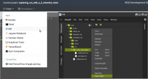
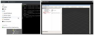
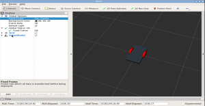
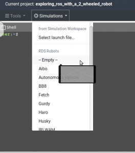
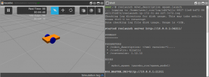
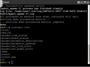
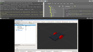
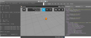
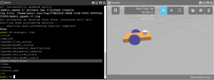
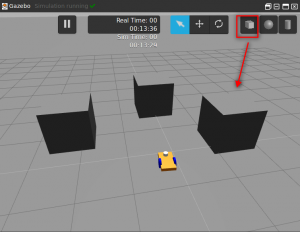
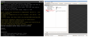
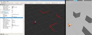

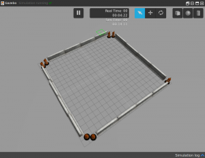
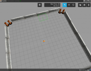
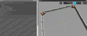
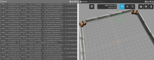
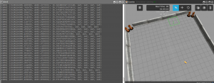
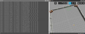
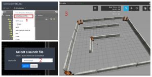
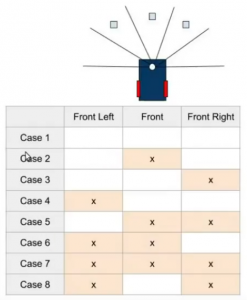
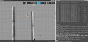
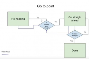
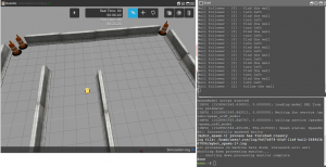
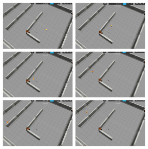
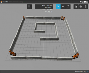
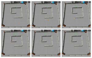
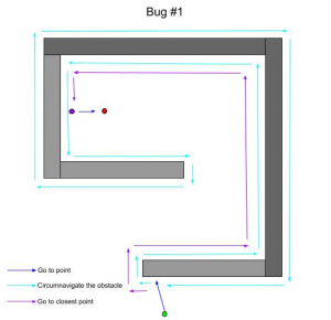
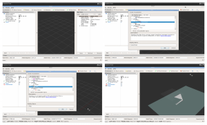
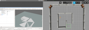
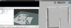



0 Comments